An Elementary Definition
Definition 1. A dynamical system is a tuple \((X, f)\) where the set \(X\) is the state space representing all possible states of the system and \(f\) is an evolution operator \(\mathbb{T}\times X\to X\), \((t, x)\mapsto f^t(x)\), on a time set \(\mathbb{T}\). If \(\mathbb{T}=\mathbb{Z}\), the system is said to be discrete, and we write \(f\) for \(f^1\), so that \(f^n\) is its \(n\)-th iterate; if \(\mathbb{T}=\mathbb{R}\), the system is said to be continuous.
Definition 2. Let \((\mathbb{R}^d, f)\) be a discrete system with a fixed point \(p\). Fix an open ball with radius \(r\). Suppose \(\forall \epsilon > 0\) there exists \(N \in \mathbb{N}\) such that \(\forall n > N\) we have
\[f^n(B_{r}^o(p)) \subseteq B_{\epsilon}^o(p)\]then \(p\) is called a sink or attracting fixed point.
Suppose \(\forall \epsilon > 0\) there exists \(N \in \mathbb{N}\) such that \(\forall n > N\) we have
\[f^n(B_{\epsilon}^o(p)) \cap B_{\epsilon}^o(p) = \{p\}\]then \(p\) is called a source or repeller.
Note this just means a sink is when we can shrink any open ball around it to an arbitrarily small open ball by taking sufficiently large steps. Similarily source is a point when we can expand arbitrary open ball so that everything except the point itself goes outside the ball by taking sufficiently large steps.
Example 1. (Hénon map) Consider the parametrized non-linear, discrete time system:
\[\begin{align*} x_{n+1}&=a-x_n^2 + by_n \\ y_{n+1}&=x_n \end{align*}\]We can simulate the action of Hénon map by starting with a grid of points and apply them for many iterations. Writing a small julia function:
compute_attractor function in julia
function compute_attractor(a, b; N=1000, T=1000, h=100, w=100)
    states = zeros(N, N, 2)
    for i = 1:N
        for j = 1:N
            for t = 1:T
                if t == 1
                    states[i,j,1] = -h/2 + (i-1)*h/N
                    states[i,j,2] = -w/2 + (j-1)*w/N
                else
                    x = states[i,j, 1]
                    y = states[i,j, 2]
                    if (abs(x) < 1e2) && (abs(y) < 1e2)
                        states[i,j, 1] = a - x^2 + b*y
                        states[i,j, 2] = x
                    else
                        states[i, j, 1] = Inf
                        states[i, j, 2] = Inf
                    end
                end
            end
        end
    end
    return states
end
For \(a=1.4, b=0.3\), the image looks like:
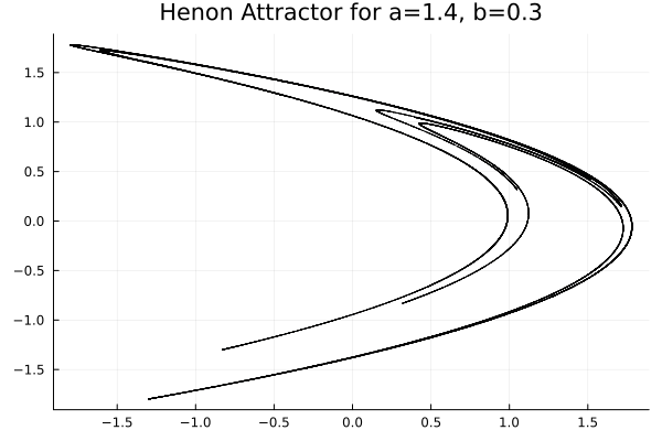
This gets an approximation of the attractor, which is a generalization of fixed point.
Definition 3. Let \((X,f)\) be a dynamical system where \(X\) is compact and equipped with a topology and \(f\) is continuous. A compact subset \(C\subseteq X\) is called an attractor if there is an open set \(U\subseteq X\) such that:
- \[f(\overline{U})\subseteq U\]
- \[C=\bigcap_{k=0}^{\infty} f^k(U)\]
Proposition 1. \(\forall x\in U\), \(x\) converges to the set \(C\) in the following sense: \(\forall V \supseteq C\) that is open, \(\exists N>0\) such that \(\forall n > N\), \(f^n(x)\in V\).
proof
Proof: First we note that the set \(f^n(\overline{U})\) forms a decreasing sequence
\[\overline U \supseteq f(\overline U ) \supseteq f^2(\overline U ) \cdots\]Since \(f(\overline U ) \subseteq U \subseteq \overline{U}\).
This implies the complement forms an increasing sequence:
\[X\setminus \overline U \subseteq X \setminus f(\overline U ) \subseteq X \setminus f^2(\overline U ) \cdots\]Now we claim that \(X=V \cup \bigcup_{k=0}^{\infty} X \setminus f^k(\overline{U})\). This can be shown:
- \[x\in C \Longrightarrow x\in V\]
- \(x \notin C \Longrightarrow \exists m\), \(x\notin f^m(U) \Longrightarrow x \in \bigcup_{k=0}^{\infty} X \setminus f^k(\overline{U})\)
By compactness of \(X\), it has a finite subcover. Hence there exists some \(N>0\) such that:
\[X = V\cup \bigcup_{k=0}^{N} X \setminus f^k(\overline{U})\]However, \(X \setminus f^k(\overline{U})\) is increasing hence
\[X = V\cup (X \setminus (f^n(\overline{U})) )\quad \forall n \geq N\]Now suppose \(x\in U \Longrightarrow x \in \overline{U}\), \(f^n(x) \in f^{n}(\overline{U})\) hence by the decomposition above \(f^n(x)\) must be in \(V\).\(\blacksquare\)
Now let’s see some continous-time examples
Example 2. Consider the undampened pendulum equation: \(\frac{d^2\theta}{dt^2} + \sin(\theta)=0\) which, with \(x = \theta\) and \(y = \frac{d\theta}{dt}\), can be rewritten as:
\[\frac{d}{dt} \begin{bmatrix} x \\ y \end{bmatrix} = \begin{bmatrix} y \\ -\sin(x) \end{bmatrix}\]Another example is the Lorenz system, which originates from climate sciences(metereology), which arise after applying spectral methods to solve Oberbeck-Boussinesq approximation of the Navier-Stokes equation.
Example 3.
\[\frac{d}{dt} \begin{bmatrix} x \\ y \\ z \end{bmatrix} = \begin{bmatrix} \sigma(y-x) \\ \rho x - y - xz \\ -\beta z + xy \end{bmatrix}\]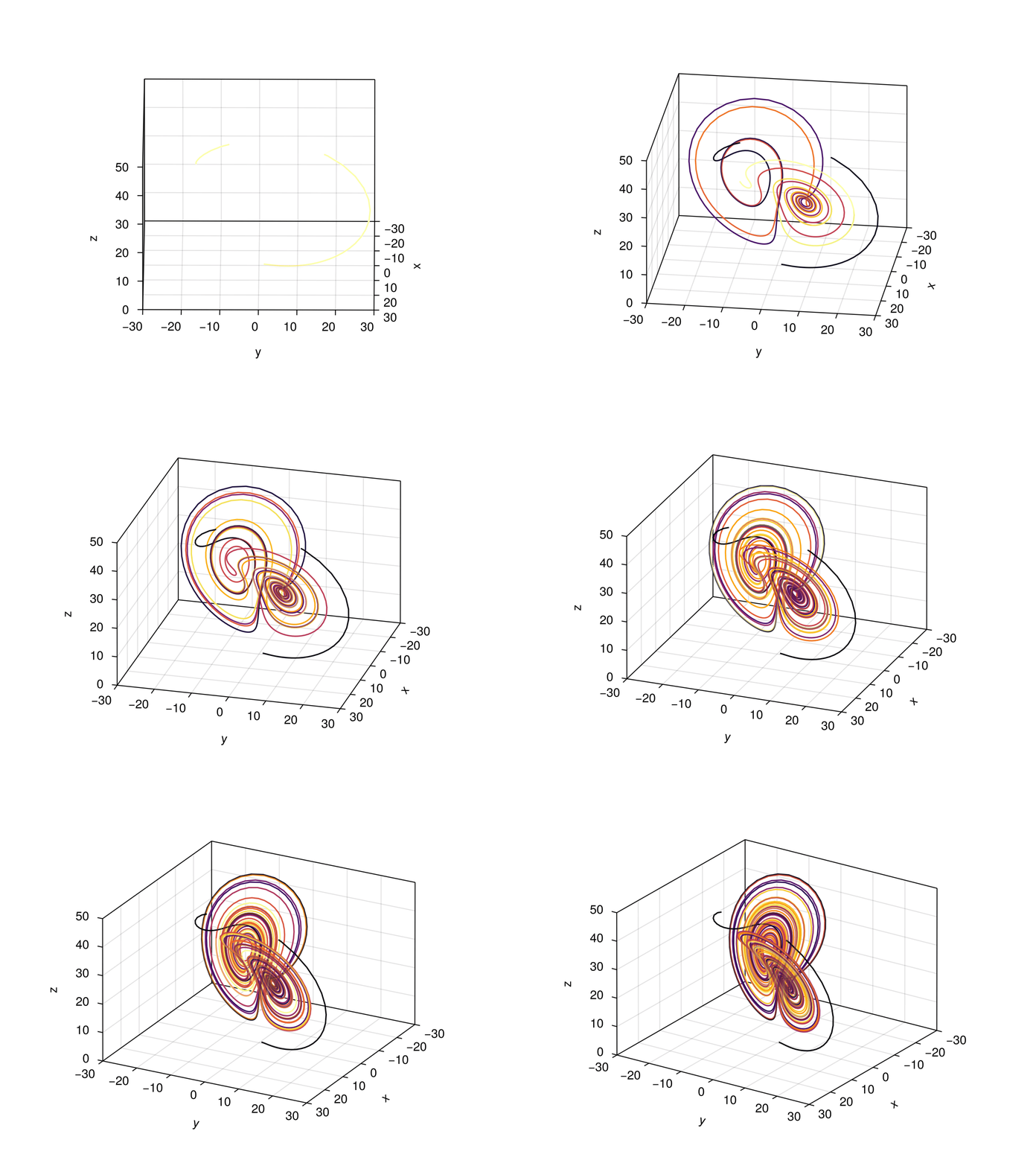
lorenz simulation in julia(modified from wiki)
import Pkg; Pkg.add("GLMakie")
using GLMakie

Base.@kwdef mutable struct Lorenz
    dt::Float64 = 0.01
    σ::Float64 = 10
    ρ::Float64 = 28
    β::Float64 = 8/3
    x::Float64 = 1
    y::Float64 = 1
    z::Float64 = 1
end

function step!(l::Lorenz)
    dx = l.σ * (l.y - l.x)
    dy = l.x * (l.ρ - l.z) - l.y
    dz = l.x * l.y - l.β * l.z
    l.x += l.dt * dx
    l.y += l.dt * dy
    l.z += l.dt * dz
    Point3f(l.x, l.y, l.z)
end

attractor = Lorenz()

points = Point3f[]
colors = Int[]


fig, ax, l = lines(points, color = colors,
    colormap = :inferno, transparency = true,
    axis = (; type = Axis3, protrusions = (0, 0, 0, 0),
              viewmode = :fit, limits = (-30, 30, -30, 30, 0, 50)))

record(fig, "assets/videos/lorenz.gif", 1:120) do frame
    for i in 1:50
        push!(points, step!(attractor))
        push!(colors, frame)
    end
    ax.azimuth[]=atan(frame/90)
    Makie.update!(l, arg1 = points, color = colors)
    l.colorrange = (0, frame)
end
Lyapuov Exponent
Consider first a discrete dynamical system \((X,f)\). We are interested in how a perturbation \(\delta x\) in the initial state \(x_0\) would impact the trajectory. By linear approximation:
\[\begin{align*} x_1' &= f(x_0 + \delta x) \\ &\approx f(x_0) + Df(x_0)\,\delta x \\ &= x_1 + Df(x_0)\,\delta x \end{align*}\]where \(x_n = f^n(x_0)\) and \(x_n'\) denote the unperturbed and perturbed states at time \(n\). Similarily:
\[\begin{align*} x_2' &= f(x_1') \\ &\approx f(x_1 + Df(x_0)\,\delta x) \\ &\approx x_2 + Df(x_1)\,Df(x_0)\,\delta x \end{align*}\]Suppose we denote \(u_n=x_n'-x_n\), by induction, we have that:
\[u_n \approx Df(x_{n-1}) \cdots Df(x_1)\, Df(x_0)\, \delta x\]Or if \(f\) is time-dependent, \(x_{k+1} = f(x_k, k)\), we have
\[u_n \approx D_x f(x_{n-1}, n-1) \cdots D_x f(x_1, 1)\, D_x f(x_0, 0)\, \delta x\]We’ll denote the product of matrices by 2
\[\boxed{H(x_0, n) := D_x f(x_{n-1}, n-1) \cdots D_x f(x_1, 1)\, D_x f(x_0, 0)}\]so that \(u_n \approx H(x_0, n)\, \delta x\); for autonomous \(f\), \(H(x_0, n) = Df(x_{n-1}) \cdots Df(x_0) = Df^n(x_0)\) by the chain rule.
Example 4. The jacobian of the Hénon map is:
\[Df(x, y) = \begin{bmatrix} -2x & b \\ 1 & 0 \end{bmatrix}\]Hence, writing the state at time \(k\) as \((x_k, y_k)\), the perturbation is simply:
\[u_n \approx \underbrace{ \begin{bmatrix} -2x_{n-1} & b \\ 1 & 0 \end{bmatrix} \cdots \begin{bmatrix} -2x_0 & b \\ 1 & 0 \end{bmatrix} }_{H((x_0, y_0), n)} \delta x\]Continuous Time
For a continuous system \(\frac{dx}{dt} = F(x, t)\) with trajectory \(x(t)\) starting at \(x_0\), a perturbation \(u(t) = x'(t) - x(t)\) with \(u(0) = \delta x\) obeys, to first order, the linear equation
\[\frac{du}{dt} = J(t)\, u, \qquad J(t) := D_x F(x(t), t),\]where \(J(t)\) is the Jacobian of \(F\) along the trajectory. Its solution defines the continuous analog of \(H\):
Definition 4. For \(t \ge 0\), let \(H(x_0, t)\) be the matrix solving
\[\frac{d}{dt} H(x_0, t) = J(t)\, H(x_0, t), \qquad H(x_0, 0) = I,\]so that \(u(t) \approx H(x_0, t)\, \delta x\). It is written as a time-ordered exponential
\[\boxed{H(x_0, t) = \mathcal{T}\exp\left(\int_0^t J(s)\, ds\right)}\]For autonomous \(F\), \(H(x_0, t) = Df^t(x_0)\), the Jacobian of the flow map.
Time-ordered Exponential. \(\mathcal{T}\exp\) is not the matrix exponential of \(\int_0^t J(s)\, ds\). Solving the equation above by repeated substitution gives the series
\[\begin{align*} H(x_0, t) &= I + \int_0^t J(s_1)H(x_0,s_1)ds_1 \\ &= I + \int_0^t J(s_1)\left( I + \int_0^{s_1} J(s_2)H(x_0,s_s)ds_2\right)ds_1 \\ &= I + \int_0^t J(s_1) ds_1 + \int_0^t \int_0^{s_1} J(s_2)H(x_0, s_2)ds_2 \\ \vdots \\ &= I + \sum_{k=1}^{\infty} \int_0^t \int_0^{s_1}\cdots \int_{0}^{s_k} J(s_1),...,J(s_k)ds_k \end{align*}\]Now consider the time-ordering \(\mathcal{T}\) permutes each product so that later times stand to the left:
\[\mathcal{T}\big[J(s_1) \cdots J(s_k)\big] = J(s_{\pi(1)}) \cdots J(s_{\pi(k)}), \qquad \pi \text{ the permutation with } s_{\pi(1)} \ge \cdots \ge s_{\pi(k)}.\]Note for each \((s_1,s_2,...)\) the \(\mathcal{T}\) enforces a possibly different order, i.e., \(\mathcal T\) is point-wise.
Now we claim that:
\[\boxed{ \sum_{k=1}^{\infty} \frac{1}{k!}\int_0^t\int_0^t ... \int_0^t \mathcal{T}(J(s_1),...,J(s_k))ds_k = \sum_{k=1}^{\infty} \int_0^t \int_0^{s_1}\cdots \int_{0}^{s_k} \mathcal T(J(s_1),...,J(s_k))ds_k }\]Editing notes: Need a proof here
However, if the jacobian \(J_j(s_j)\) commute with each other, \(\mathcal T\) would be redundant.
Some examples:
- Linear systems \(F(x) = Ax\) have \(J(s) = A\) for all \(s\), so \(H(x_0, t) = e^{tA}\).
- One-dimensional systems have scalar Jacobians, which always commute, so \(H(x_0, t) = \exp\left(\int_0^t F'(x(s))\, ds\right)\).
- Determinants turn matrices into numbers, so \(\det H\) always behaves like the scalar case. This is Liouville’s formula: \(\det H(x_0, t) = \exp\left(\int_0^t \operatorname{tr} J(s)\, ds\right)\).
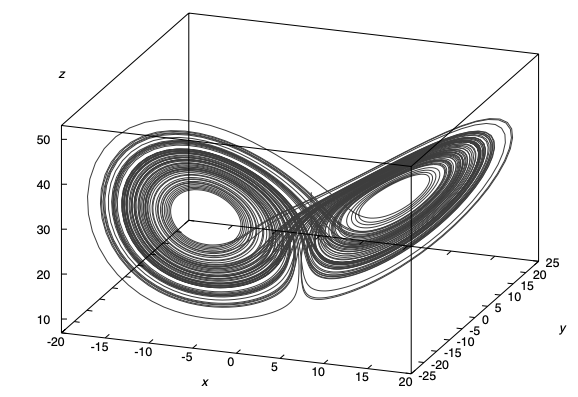
- The Lorenz system has Jacobians that do not commute at different points, so its \(H\) is a genuine time-ordered exponential.
The Oseledets Theorem
Theorem 1. (Oseledets) Let \((X, \mathcal{B}, \mu)\) be a probability space, \(f: X \to X\) a measure-preserving map, and \(T: X \to \mathbb{R}^{d \times d}\) a measurable function with \(\int_X \log^+ \Vert{}T(x)\Vert{} \, d\mu(x) < \infty\), where \(\log^+ y = \max(0, \log y)\). Write
\[T^n(x) := T(f^{n-1}(x)) \cdots T(f(x))\, T(x),\]which for \(T = Df\) is \(Df^n(x) = H(x, n)\) by the chain rule. Then for \(\mu\)-a.e. \(x\) there are an integer \(1 \le s(x) \le d\), exponents \(+\infty > \lambda_1(x) > \dots > \lambda_{s(x)}(x) \ge -\infty\) and a filtration
\[\mathbb{R}^d = V_1(x) \supsetneq V_2(x) \supsetneq \cdots \supsetneq V_{s(x)}(x) \supsetneq V_{s(x)+1}(x) = \{0\}\]such that:
- Growth rates: \(\lim_{n \to \infty} \frac{1}{n} \log \Vert{}T^n(x)\, v\Vert{} = \lambda_i(x)\) for every \(v \in V_i(x) \setminus V_{i+1}(x)\).
- Invariance along orbits: \(s\), \(\lambda_i\) and \(m_i := \dim V_i - \dim V_{i+1}\) are functions of the starting point \(x\), but they are constant along each orbit: \(\lambda_i(f(x)) = \lambda_i(x)\), and likewise for \(s\) and \(m_i\). If \(\mu\) is ergodic, they are the same for \(\mu\)-a.e. \(x\). The subspaces travel with the orbit: \(T(x)\, V_i(x) \subseteq V_i(f(x))\).
- Matrix limit: \(\Lambda(x) := \lim_{n \to \infty} \left( T^n(x)^\top T^n(x) \right)^{1/(2n)}\) exists and has eigenvalues \(e^{\lambda_i(x)}\) with multiplicities \(m_i(x)\) (where \(e^{-\infty} = 0\)); \(V_i(x)\) is the sum of the eigenspaces for \(e^{\lambda_i(x)}, \dots, e^{\lambda_{s(x)}(x)}\).
In words: fix a typical starting point \(x\) (typical for \(\mu\)) and perturb it in a direction \(v\). The perturbation grows or shrinks like \(e^{n\lambda}\), where the rate \(\lambda\) is one of finitely many values \(\lambda_1 > \dots > \lambda_s\) and depends only on the direction: it is \(\lambda_i\) exactly when \(v \in V_i(x) \setminus V_{i+1}(x)\) (item 1). A randomly chosen direction gets the largest rate \(\lambda_1\), because \(V_2(x)\) is a lower-dimensional subspace. The rates belong to the whole orbit, not just to the point \(x\) (item 2), and they are also the growth rates of the singular values of \(T^n(x)\) (item 3).
Computing the Spectrum Numerically
The theorem suggests an algorithm (Benettin et al., 1980): follow a frame of \(d\) perturbation vectors along the trajectory and measure how fast it stretches. Two problems arise if the frame is evolved naively: every column turns toward the fastest direction \(V_1 \setminus V_2\), and the entries overflow. The fix is to re-orthonormalize with a QR decomposition every few steps. The \(k\)-th diagonal entry of \(R\) is the growth of the \(k\)-th column after the first \(k-1\) directions have been removed, so its logarithm, averaged over time, converges to \(\lambda_k\).
input: vector field F, Jacobian DF, initial state x, step Δt, block length m, number of blocks N
U ← I                                  # orthonormal frame of d perturbations
S ← 0                                  # accumulated log-stretching, one entry per exponent
run x forward for a while so it lands on the attractor
repeat N times:
    repeat m times:                    # one Euler step of x and of the frame
        x, U ← x + Δt F(x),  U + Δt DF(x) U
    Q, R ← qr(U)                       # U = QR, Q orthonormal, R upper triangular
    S ← S + log |diag(R)|              # how much each direction stretched
    U ← Q                              # restart from an orthonormal frame
return S / (N m Δt)                    # λ_1, ..., λ_d
The frame update \(U \leftarrow U + \Delta t\, DF(x)\, U = (I + \Delta t\, J)\, U\) is one Euler step of \(\frac{d}{dt}H = JH\), so between re-orthonormalizations \(U\) tracks \(H(x_0, t)\) applied to the frame.
Lyapunov spectrum of the Lorenz system in julia (here R = ρ, b = β)
# A script to compute the lyapunov spectrum for the lorenz system
# @ author : Haoyu Tang

using LinearAlgebra

Base.@kwdef mutable struct State
    x::Float64 = 1
    y::Float64 = 1
    z::Float64 = 1
    U::Matrix{Float64} = Matrix{Float64}(I,3,3)
end

Base.@kwdef mutable struct Lorenz
    dt::Float64 = 0.001
    σ::Float64 = 10
    R::Float64 = 28
    b::Float64 = 8/3
    v::State = State()
end

function compute_attractor!(L::Lorenz; N=100)
    v, σ, R, b, dt = L.v, L.σ, L.R, L.b, L.dt
    for T = 1:N
        v.x += σ * (v.y - v.x) * dt
        v.y += (R * v.x - v.y - v.x * v.z) * dt
        v.z += (- b * v.z + v.x * v.y) * dt
    end
end

function rhs(L::Lorenz)
    v, σ, R, b = L.v, L.σ, L.R, L.b
    x, y, z, U = v.x, v.y, v.z, v.U
    J = [-σ  σ  0 ; (R - z)  -1 -x ; y x -b]
    dX = [σ * (y - x), R * x - y - x * z, - b * z + x * y]
    dU = J * U
    return hcat(dX, dU)
end

function benettin!(L::Lorenz; block_size=1, total_blocks=1_000_000)
    # set up accumulator for lyapunov exponent
    S = [0 0 0]

    # integrate to get an approximation of the trajectory
    compute_attractor!(L)

    dt = L.dt
    v = L.v

    for n = 1:total_blocks
        # euler step for block_size steps
        for t = 1:block_size
            dv = rhs(L)
            v.x += dv[1, 1] * dt
            v.y += dv[2, 1] * dt
            v.z += dv[3, 1] * dt
            v.U += dv[:, 2:4] * dt
        end

        # reorthonormalization
        q, r = qr(v.U)

        # adjust sign
        sign_vector = Diagonal(sign.(diag(r)))
        q = q * sign_vector
        r = r * sign_vector

        v.U = q
        S += log.(diag(r)')
    end
    return S ./ (total_blocks * block_size * dt)
end

L = Lorenz()
λ = benettin!(L)

expected_sum = -(L.σ + L.b + 1)
computed_sum = sum(λ)

diff = (abs(expected_sum - computed_sum))/abs(computed_sum) * 100
println()
print("Expecting $expected_sum, got $computed_sum, error = $diff %")
println()
show(stdout, "text/plain", λ)
With \(\Delta t = 0.001\) over \(1000\) time units this prints \((\lambda_1, \lambda_2, \lambda_3) \approx (0.906, 0.001, -14.608)\), close to the reference values \((0.906, 0, -14.572)\). Three checks tell us whether to trust the result:
- The sum is \(-(\sigma + 1 + \beta)\). The frame’s volume is \(\lvert\det U\rvert\), which grows like \(e^{(\lambda_1 + \lambda_2 + \lambda_3)t}\). By Liouville’s formula it also equals \(\exp\left(\int_0^t \operatorname{tr} J\, ds\right)\), and \(\operatorname{tr} J = -\sigma - 1 - \beta\) at every point. So the sum must be \(-(\sigma + 1 + \beta) \approx -13.667\). The code gives \(-13.70\): the gap comes from Euler’s method and shrinks with \(\Delta t\). This check only sees the diagonal of \(J\), so passing it does not mean the individual exponents are right.
- One exponent is \(0\). A perturbation along the flow direction \(F(x)\) is just a shift in time along the same trajectory (\(H(x, t)\, F(x) = F(f^t(x))\)), so it neither grows nor shrinks exponentially. Every flow whose attractor is not a fixed point has this zero exponent.
- A positive exponent means chaos. If \(\lambda_1 > 0\), two nearby initial states separate like \(\lvert\delta x\rvert\, e^{\lambda_1 t}\), so an error of size \(\delta\) grows to the size \(L\) of the attractor after about \(\frac{1}{\lambda_1}\log\frac{L}{\delta}\) time units. After that, prediction is impossible. The attractor is bounded, so this stretching must be accompanied by folding, which is what produces its fractal structure. This sensitive dependence on initial conditions on a bounded attractor is what we call chaos. For Lorenz, \(1/\lambda_1 \approx 1.1\) time units: each extra digit of precision in the initial state buys only about \(2.5\) more time units of prediction.