The Impact of Ocean Basin Geometry on ENSO Frequency
May 15, 2026
Acknowledgement This project is joint-work with August Zheng and is our ATMS 507 final project. August provided very detailed and execellent literature review on the topic and provided great physical insights into our discussions. We also thank Professor Gan Zhang for key feedbacks and access to L40S on the keeling cluster.
The El Niño–Southern Oscillation (ENSO) is regulated by equatorial waves: Kelvin waves carry thermocline anomalies east, Rossby waves carry them back west, and the time these waves need to cross the Pacific sets the ocean’s memory. So the frequency should depend on the basin width \(L_x\), at least in idealized models. We test this in the simplest such model, the linear shallow-water equations on an equatorial \(\beta\)-plane, by simulating a range of basin widths and measuring the dominant frequency of the eastern thermocline anomaly.
Equatorial Waves
Why should the width matter? Matsuno (1966) answered this by finding the free waves of the linear equatorial shallow-water equations. Scale lengths by the equatorial deformation radius \(L_{eq} = \sqrt{c/\beta}\) and times by \(T = 1/\sqrt{c\beta}\), where \(c = \sqrt{g'H}\) is the gravity-wave speed. The equations become
\[\begin{align*} u_t - y v + \phi_x &= 0, \\ v_t + y u + \phi_y &= 0, \\ \phi_t + u_x + v_y &= 0, \end{align*}\]with \(\phi\) the (scaled) thermocline displacement. Since the coefficients depend only on \(y\), look for waves travelling in \(x\):
Wave ansatz For wavenumber \(k\) and frequency \(\omega\),
\((u, v, \phi) = \big(\hat u(y), \hat v(y), \hat\phi(y)\big)\, e^{i(kx - \omega t)}.\)
Substituting gives three ODEs in \(y\):
\[\begin{align*} -i\omega \hat u - y\hat v + ik\hat\phi &= 0, \\ -i\omega \hat v + y\hat u + \hat\phi' &= 0, \\ -i\omega \hat\phi + ik\hat u + \hat v' &= 0. \end{align*}\]The first equation is algebraic: \(\hat u = (ik\hat\phi - y\hat v)/(i\omega)\). Putting it into the third and solving for \(\hat\phi\) gives
\[\hat\phi = \frac{i\,(\omega \hat v' - k y \hat v)}{k^2 - \omega^2},\]and putting both into the second equation, the terms in \(\hat v'\) cancel and we are left with a single equation for \(\hat v\):
\[\hat v'' + \left(\omega^2 - k^2 - \frac{k}{\omega} - y^2\right)\hat v = 0.\]This is the Schrödinger equation of the quantum harmonic oscillator, \(\hat v'' + (\lambda - y^2)\hat v = 0\). Its solutions stay bounded as \(y \to \pm\infty\) (the waves are trapped at the equator) only for \(\lambda = 2n + 1\), with \(\hat v = H_n(y)\, e^{-y^2/2}\) for the Hermite polynomials \(H_n\).
Proposition (Dispersion relation) Equatorially trapped waves satisfy
\[\omega^2 - k^2 - \frac{k}{\omega} = 2n + 1, \qquad n = 0, 1, 2, \dots\]In addition, \(\hat v \equiv 0\), \(\omega = k\) is the Kelvin wave, which travels east at speed \(c\).
For slow waves, \(\omega^2\) is negligible and the relation gives \(\omega = -k/(k^2 + 2n + 1)\): these are the Rossby waves, with westward phase speed. In dimensional form,
\[\boxed{c_R = -\frac{\beta}{k^2 + \frac{\beta}{c}(2n + 1)}}\]For long waves (\(k \to 0\)) this is \(c_R = -c/(2n+1)\), so the gravest (\(n = 1\)) Rossby wave is three times slower than the Kelvin wave.
What to expect. A Kelvin wave crossing the basin eastward and a Rossby wave returning westward take \(L_x/c + 3L_x/c = 4L_x/c\). With the parameters below (\(c \approx 1.6\) m/s), a \(12\,000\) km basin gives about \(0.96\) years. This transit-time picture predicts a frequency close to one cycle per year that scales like \(L_x^{-1}\).
Equations of Motion
We simulate the ocean part of the linear shallow-water system on the equatorial \(\beta\)-plane, with Rayleigh friction \(r\) and a zonal trade-wind stress \(\tau^{(x)}\) (meridional stress is neglected):
\[\begin{align*} \partial_t u &= \beta y v - g'\,\partial_x h - r u + \tau^{(x)}, \\ \partial_t v &= -\beta y u - g'\,\partial_y h - r v, \\ \partial_t h &= -H\,(\partial_x u + \partial_y v). \end{align*}\]Here \(g' = g\,\Delta\rho/\rho_0\) is the reduced gravity, gravity corrected for buoyancy across the thermocline. The initial thermocline anomaly is an equatorial bump plus a zonal tilt,
\[h(x, y, 0) = \exp\left(-\frac{c_1 y^2}{R^2}\right) + c_2 x.\]| Parameter | Symbol | Value |
|---|---|---|
| Meridional gradient of the Coriolis parameter | \(\beta\) | \(2.28 \times 10^{-11}\ \mathrm{m^{-1}\,s^{-1}}\) |
| Reduced gravity | \(g'\) | \(0.05\ \mathrm{m\,s^{-2}}\) |
| Rayleigh friction | \(r\) | \(10^{-7}\ \mathrm{s^{-1}}\) |
| Mean thermocline depth | \(H\) | \(50\ \mathrm{m}\) |
| Gravity-wave speed | \(c = \sqrt{g'H}\) | \(\approx 1.58\ \mathrm{m\,s^{-1}}\) |
| Equatorial deformation radius | \(L_{eq} = \sqrt{c/\beta}\) | \(\approx 263\ \mathrm{km}\) |
Numerical Method
The simplest discretization is the method of lines: replace spatial derivatives with finite differences and integrate the resulting system of ODEs for the grid values \((u_{i,j}(t), v_{i,j}(t), h_{i,j}(t))\) in time. Two problems came up, each with its own fix:
- the checkerboard problem, solved by the Arakawa C-grid;
- a drift of the mean thermocline depth, solved by a sponge layer and centering.
The Checkerboard Problem
On an A-grid, \(u\), \(v\) and \(h\) all live at cell centres and derivatives are central differences, e.g. \(\partial_x h \approx (h_{i+1,j} - h_{i-1,j})/(2\Delta x)\). To see what goes wrong, take the 1D toy problem
\[\partial_t u = -\partial_x h, \qquad \partial_t h = -0.01\,\partial_x u,\]discretized as
\[\frac{du_i}{dt} = -\frac{h_{i+1} - h_{i-1}}{2\Delta x}, \qquad \frac{dh_i}{dt} = -0.01\,\frac{u_{i+1} - u_{i-1}}{2\Delta x},\]on 7 cells, with a unit bump of \(h\) in the middle, \(u = 0\) and \(\partial_x h = 0\) at the walls, and \(\Delta x = \Delta t = 1\).
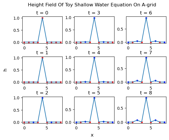
Every other cell (red) never changes. The reason is visible in the stencil: \(du_i/dt\) uses only \(h_{i\pm1}\), and \(dh_i/dt\) uses only \(u_{i\pm1}\). So \(h\) on even cells talks only to \(u\) on odd cells and vice versa: the grid splits into two independent sublattices, and a wave started on one never reaches the other.
A Fourier mode \(h_i = e^{ik i\Delta x}\) makes this quantitative. The central difference multiplies it by \(i\sin(k\Delta x)/\Delta x\), so the discrete waves obey
\[\omega_A = \frac{c\,\sin(k\Delta x)}{\Delta x},\]which vanishes at \(k\Delta x = \pi\): the checkerboard mode \(h_i = (-1)^i\) has zero discrete gradient, feels no pressure force and never moves.
The Arakawa C-Grid
The C-grid keeps \(h\) at cell centres but moves \(u\) to the east/west faces and \(v\) to the north/south faces:
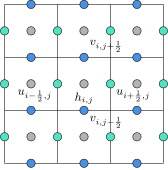
Each derivative is now a difference across one cell, taken exactly where it is needed:
\[\begin{align*} \frac{du_{i+\frac12,j}}{dt} &= \beta y_j\, \bar v_{i+\frac12,j} - g'\,\frac{h_{i+1,j} - h_{i,j}}{\Delta x} - r\,u_{i+\frac12,j} + \tau^{(x)}, \\ \frac{dv_{i,j+\frac12}}{dt} &= -\beta y_{j+\frac12}\, \bar u_{i,j+\frac12} - g'\,\frac{h_{i,j+1} - h_{i,j}}{\Delta y} - r\,v_{i,j+\frac12}, \\ \frac{dh_{i,j}}{dt} &= -H\left(\frac{u_{i+\frac12,j} - u_{i-\frac12,j}}{\Delta x} + \frac{v_{i,j+\frac12} - v_{i,j-\frac12}}{\Delta y}\right), \end{align*}\]where \(\bar u\), \(\bar v\) are four-point averages that bring the other velocity component to the right face for the Coriolis term. In the Fourier picture the one-cell difference multiplies a mode by \(2i\sin(k\Delta x/2)/\Delta x\), so
\[\omega_C = \frac{2c\,\sin(k\Delta x/2)}{\Delta x},\]which is strictly positive for \(0 < k\Delta x \le \pi\): no mode is left behind. It is also more accurate. Compared with the exact \(\omega = ck\), \(\omega_A \approx ck\,(1 - k^2\Delta x^2/6)\) while \(\omega_C \approx ck\,(1 - k^2\Delta x^2/24)\), four times smaller error. On the toy problem the bump now spreads to every cell:
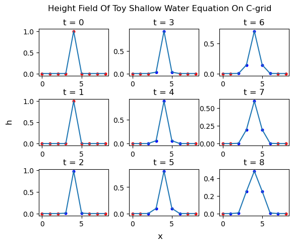
This matters for cost. On the A-grid, the only defense against the checkerboard is a very fine grid, which with an explicit time step forces a tiny \(\Delta t\): an 800-day simulation took 45–60 minutes in Python. On the C-grid a coarser grid and a larger step suffice, and the same run takes under 3 minutes.
A-grid toy loop in python
def a_grid_toy(T=6, N=7):
    h = np.zeros((T, N+2))
    h[0, (N+1)//2] += 1.0
    u = np.zeros((T, N+2))
    for t in range(1, T):
        dh_dx = np.array([(h[t-1, i+1] - h[t-1, i-1])/2 for i in range(1, N+1)])
        du_dx = np.array([(u[t-1, i+1] - u[t-1, i-1])/2 for i in range(1, N+1)])
        h[t, 1:N+1] = h[t-1, 1:N+1] - 0.01 * du_dx
        u[t, 1:N+1] = u[t-1, 1:N+1] - dh_dx
    return h, u
Mean Drift of the Thermocline
The domain is a strip of the open ocean, but the Neumann condition \(\partial_y h = 0\) at the northern and southern edges acts as a solid wall: waves reflect back instead of leaving. Under constant trade-wind forcing, energy then accumulates and the mean thermocline depth drifts upward, which is unphysical. Two adjustments fix this.
-
Sponge layer. Within a distance \(d_{\text{sponge}}\) of the northern and southern edges, the Rayleigh friction grows quadratically towards the boundary,
\[r(y) = r_{\max}\left(\frac{|y| - (L_y/2 - d_{\text{sponge}})}{d_{\text{sponge}}}\right)^2,\]so waves are absorbed before they reach the wall, as they would be by leaving the domain.
-
Centering and capping. The sponge does not drain all the energy, so the domain mean \(h_{\text{mean}} = \frac{1}{L_xL_y}\sum_{i,j} h_{i,j}\) still creeps up. Inspired by Manabe’s convective adjustment, after every time step we remove it and cap extreme values:
\[h_{i,j} \leftarrow h_{i,j} - h_{\text{mean}}, \qquad h_{i,j} \leftarrow \min\big(\max(h_{i,j}, -20), 20\big).\]
Results
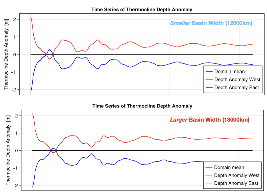
We simulate basin widths from \(11\,000\) to \(13\,000\) km in steps of \(250\) km. In both the narrow and the wide basin, the thermocline tilts as expected under easterly trade winds (deeper in the west, shallower in the east) and the anomalies oscillate while settling. The domain mean stays at zero, so the drift correction works.
The power spectrum of the eastern thermocline anomaly has a dominant peak between about \(0.7\) and \(0.9\) cycles per year, which shifts to lower frequency as the basin widens.
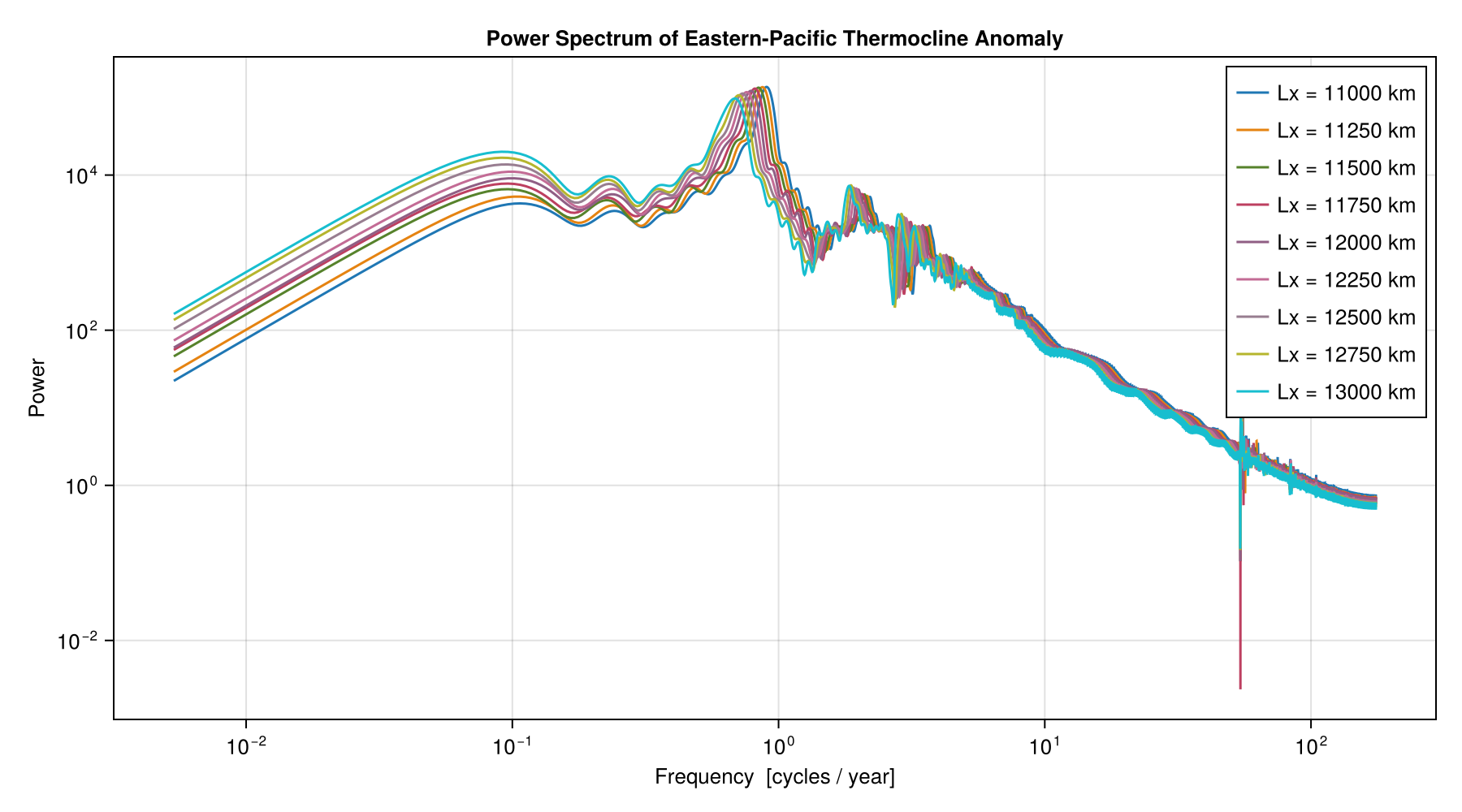
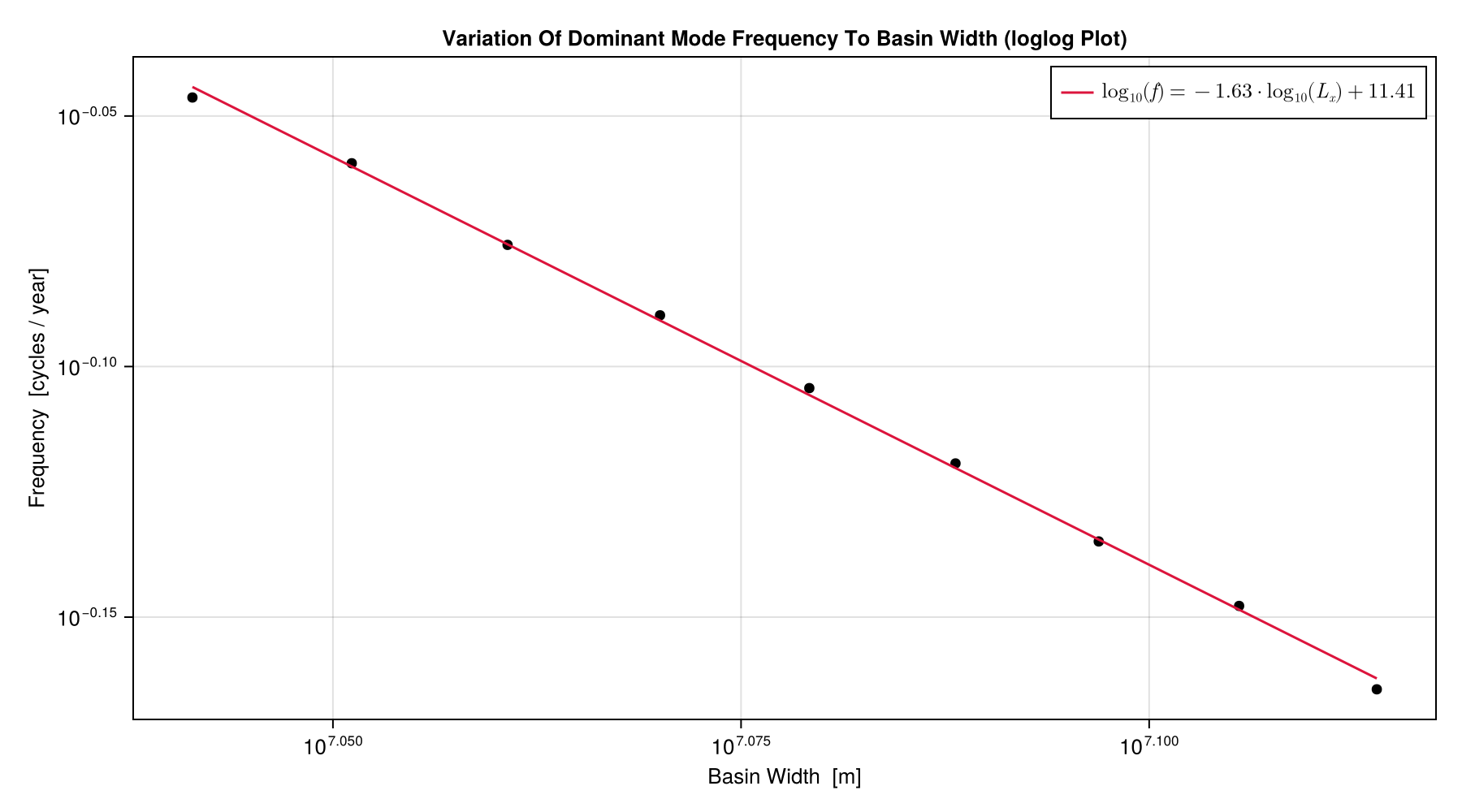
Plotting the peak frequency \(f\) against the width on log-log axes gives an almost straight line,
\[\log_{10} f = -1.63\,\log_{10} L_x + 11.41,\]that is, \(f \propto L_x^{-1.63}\).
The magnitude matches the transit-time estimate: at \(L_x = 12\,000\) km the fit gives \(f \approx 0.74\) cycles per year, against about \(1\) from \(4L_x/c\). The dependence is steeper than the \(L_x^{-1}\) that pure wave transit predicts, so wave crossing time alone does not set the frequency, even in this linear model.
In Context
Our experiment isolates one mechanism, ocean wave adjustment, from the full coupled problem. In the ENSO literature, the Bjerknes feedback amplifies anomalies while this slow ocean adjustment supplies the memory that carries the system from one phase to the next (Neelin et al., 1998), so geometry should matter, but not alone. Idealized coupled simulations find that the response to basin width is strong but non-monotonic, with regime changes between narrow, Pacific-like and wide basins (Dommenget & Hutchinson, 2025), and in the smaller Atlantic the same ingredients show up in the seasonal cycle rather than as a free interannual oscillation (Burls et al., 2011). This is why we fit an empirical relation to discrete simulations instead of assuming a scaling law, and why our result should be read as a baseline for the wave-adjustment part of the ENSO timescale, not a theory of the real ENSO period.
References
- T. Matsuno (1966). Quasi-geostrophic motions in the equatorial area. J. Meteor. Soc. Japan 44(1), 25–43. doi:10.2151/jmsj1965.44.1_25
- J. D. Neelin et al. (1998). ENSO theory. J. Geophys. Res. 103(C7), 14261–14290. doi:10.1029/97JC03424
- N. J. Burls, C. J. C. Reason, P. Penven, S. G. Philander (2011). Similarities between the tropical Atlantic seasonal cycle and ENSO: an energetics perspective. J. Geophys. Res. 116, C11010. doi:10.1029/2011JC007164
- D. Dommenget, D. K. Hutchinson (2025). El Niño southern oscillation and tropical basin interaction in idealized worlds. Climate Dynamics 63, 274. doi:10.1007/s00382-025-07759-9
- S. Abhik et al. (2025). Stronger and prolonged El Niño–Southern Oscillation in the Early Eocene warmth. Nature Communications 16, 4053. doi:10.1038/s41467-025-59263-7
- Z. Lu, Z. Liu, J. Zhu, K. M. Cobb (2018). A review of paleo El Niño–Southern Oscillation. Atmosphere 9, 130. doi:10.3390/atmos9040130