Eigenvector Preferential Attachment Networks
December 1, 2025
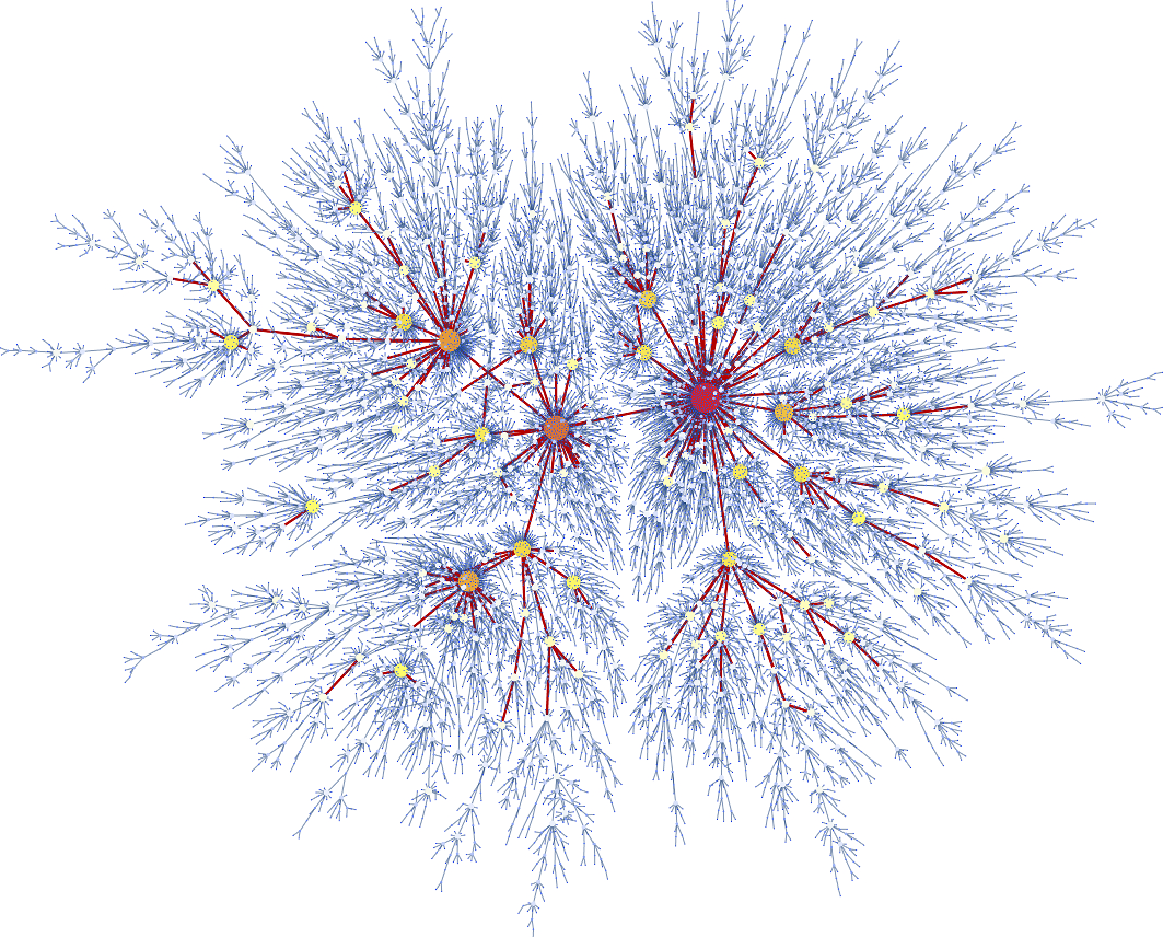
Acknowledgements: Joint work with Arha Gatram, Srujan Roplekar, and Shuwei Zhang, under graduate mentors Jaya Manthripragada and Taegu Kang, and faculty mentor Dr. Neeladri Maitra, as part of the Illinois Mathematics Lab.
Introduction
The eigenvector preferential attachment network (EPAN), introduced by Adami et al. from the physics community, is a modification of a popular model for the growth of real-world networks.
“Preferential attachment” refers to a wide class of dynamic graphs studied in random graph theory — the study of statistical properties of randomly generated graphs. Preferential attachment was first proposed by Barabási and Albert. “Eigenvector” refers to Adami et al.’s modification, where the spectral properties of the graph, rather than its degree sequence, determine its growth.
Both models are instances of a dynamic network: a description of a real-world network as the long-time limit of a graph that continually adds, removes, or modifies edges and vertices. Informally, we treat a dynamic network as a graph-valued, discrete-time stochastic process \(\{G_n\}, n\in \mathbb{N}\), with a suitable distribution for \(G_{n+1}\) conditional on \(G_n\).
Classical preferential attachment
Barabási–Albert preferential attachment (BA) is the classical model for the dynamics of real-world networks: at each discrete time step a new vertex is added and randomly attaches to an existing vertex according to the “rich get richer” principle — attachment probability proportional to degree. Writing \(G_n\) for the \(n\)-th graph with vertices \(1,\dots,n\), the new vertex \(n+1\) attaches with
\[\mathbb{P}(n+1 \text{ attaches to } i) = \frac{\deg(i)}{\sum_{j=1}^n \deg(j)}\]where exactly \(m\) of the possible edges \((i, n+1)\) are added to form \(G_{n+1}\).
Eigenvector preferential attachment
EPAN captures the global influence of a vertex by determining attachment probabilities through eigenvector centrality rather than degree. This requires first confirming the model is well-defined.
Corollary of the Perron–Frobenius theorem. Let \(G\) be a connected, undirected graph. Then its adjacency matrix \(A\) has a positive maximal eigenvalue \(\rho\) of multiplicity 1, and the corresponding eigenvector \(v_{\max}\) has strictly positive entries.
Every graph \(G_n\) produced by the (undirected) BA process is connected, and EPAN adds only undirected, unweighted edges over the same sample space — so the Perron–Frobenius theorem applies at every step.
Definition (eigenvector centrality). Let \(G\) be a connected, undirected graph. The eigenvector centrality of vertex \(i \in V(G)\) is the \(i\)-th coordinate of the \(\ell_1\)-normalized Perron–Frobenius eigenvector \(v_{\max}\).
EPAN replaces the BA preference function with
\[\mathbb{P}(n+1 \text{ attaches to } i) = v_i, \qquad v = \ell_1\text{-normalized Perron–Frobenius eigenvector of } A(G_n)\]As before we fix \(m \in \mathbb{N}\): the new vertex samples \(m\) existing vertices without replacement, weighted by \(v\). The Perron–Frobenius corollary shows this is well-defined at every step — though note that \(\big(v_i(G_n)\big)_{i=1}^n\) is itself random, and changes over time both in value and in dimension.
Proposition. For all \(n \in \mathbb{N}\), \(G_n^{(m)}\) is a tree if and only if \(m=1\). For all \(m>1\), \(G_n^{(m)}\) is connected and cyclic.
Proof (induction on \(n\)). If \(m=1\), \(G_2 = K_2\) is a tree. Suppose \(G_n\) is a tree; form \(G_{n+1}\) by attaching vertex \(n+1\) with a single edge to some vertex of \(G_n\). \(G_{n+1}\) is clearly connected, so it remains to show it is acyclic.
Every pair in \(V(G_n)\) still has a unique path between them in \(G_{n+1}\): it must equal the unique minimal-length path in \(G_n\), since any alternate path would have to enter and leave through vertex \(n+1\)’s single edge and so could not be minimal.
For a minimal path \(p_{n+1,v}\) between \(n+1\) and \(v \in V(G_n)\), write \(u\) for the unique vertex adjacent to \(n+1\). Then \(p_{n+1,v} = \lbrace n+1,u\rbrace \cdot p_{u,v}\), and since \(p_{u,v}\) is unique, so is \(p_{n+1,v}\). Since \(G_{n+1}\) is undirected with a unique minimal-length path between every pair of vertices, it is a tree.
If \(m>1\), the seed graph \(G_{m+1}=K_{m+1}\) already contains a cycle; since edges are never removed, \(G_n\) remains cyclic (and connected) for all \(n \ge m+1\). \(\blacksquare\)
Quantities of interest
Since preferential attachment models large-scale networks, most properties are studied asymptotically as \(n \to \infty\), and since real-world network data is extremely high-dimensional, we rely on a handful of summary statistics.
Height and diameter. For a tree \(G\) rooted at \(r\), height is \(\max_{u \in V} d(u,r)\); the diameter of any graph is \(\max_{u,v \in V} d(u,v)\) — both summarize how “spread out” the graph is. For \(m=1\) classical BA preferential attachment is known to have logarithmic height and diameter.
Degrees. One of the most common ways to summarize a large graph is its degree distribution.
Definition. Let \(\lbrace G_n\rbrace\) be a random graph sequence and \(U_n\) a uniformly chosen vertex of \(G_n\). Write \(D_n = \deg(U_n)\) and \(F_n(k) = \mathbb{P}(D_n = k)\). If \(F_n(k) \to p_k\) for some pmf \((p_k)_{k \ge 0}\), then \(k \mapsto p_k\) is the asymptotic degree distribution of \(\lbrace G_n\rbrace\).
Bollobás et al. rigorously confirmed Barabási–Albert’s conjecture that BA preferential attachment has a power-law degree distribution with exponent \(3\); the maximal degree in BA is of order \(n^{1/2}\).
Spectral properties. EPAN differs from prior dynamic-network models by making eigenvalues and eigenvectors part of the graph’s definition, not just an object to study after the fact. This intermingling of random-graph theory and spectral graph theory means there are comparatively few off-the-shelf tools for a fully rigorous treatment — which is exactly the gap this project tries to narrow.
Results and open problems
We simulated EPAN for \(m=1\) (tree case) and \(m=2\) (cyclic case) and organized the recurring empirical phenomena into eight concrete open problems. Throughout, \(G_t^{(m)}\) is the EPAN at “time” \(t\) (so \(\lvert V(G_t^{(m)}) \rvert = t+m+1\)), and \(\deg_t(v)\) is the degree of \(v\) in \(G_t^{(m)}\).
Superhub: existence, uniqueness, and persistence
A central structural feature of EPANs is the emergence of a single, exceptionally high-degree vertex (the “superhub”) — reported by Adami et al. for \(m=1\), and one we observe for \(m=2\) as well.
Definition (superhub). For a finite graph \(G\), \(v_{\mathrm{SH}}(G) \in \arg\max_{v \in V(G)} \deg(v)\). If the maximizer is unique, we identify \(v_{\mathrm{SH}}(G)\) with it.
Problem 1 (existence and uniqueness). Show that for fixed \(m \in \lbrace 1,2\rbrace\), with probability tending to \(1\) as \(t \to \infty\), the degree maximizer is unique:
\[\mathbb{P}\Big(\exists!\, v \in V(G_t^{(m)}): \deg_t(v) = \max_u \deg_t(u)\Big) \to 1.\]Problem 2 (persistence). Once the superhub appears, our simulations strongly suggest it stays the superhub forever. Let \(T_{\mathrm{lock}}\) be the random time after which the superhub’s identity stops changing:
\[T_{\mathrm{lock}} := \inf\Big\{t_0:\ v_{\mathrm{SH}}(G_t^{(m)}) = v_{\mathrm{SH}}(G_{t_0}^{(m)})\ \ \forall t \ge t_0\Big\}.\]Prove \(T_{\mathrm{lock}} < \infty\) with high probability, and quantify the tail behavior of \(T_{\mathrm{lock}}\).
Superhub degree scaling
Adami et al. reported — and we replicate — that for \(m=1\) the superhub degree grows on the order \(t^{2/3}\). For \(m=2\) we observe a similar scaling for the superhub, while typical high-degree non-superhub vertices scale closer to \(t^{1/3}\).
Problem 3 (correct order of the superhub degree). For fixed \(m \in \lbrace 1,2\rbrace\), determine exponents \(\alpha_m\) and constants (or slowly-varying corrections) such that
\[\deg_t\!\left(v_{\mathrm{SH}}(G_t^{(m)})\right) = t^{\alpha_m + o(1)} \quad \text{as } t \to \infty,\]justifying (or refuting) the empirical scaling \(\alpha_1 = \alpha_2 = 2/3\).
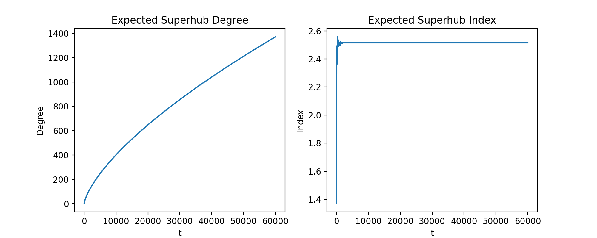 Superhub degree and index for \(m=1\). The log–log plot shows \(\deg(v_{\mathrm{SH}}) \approx t^{2/3}\).
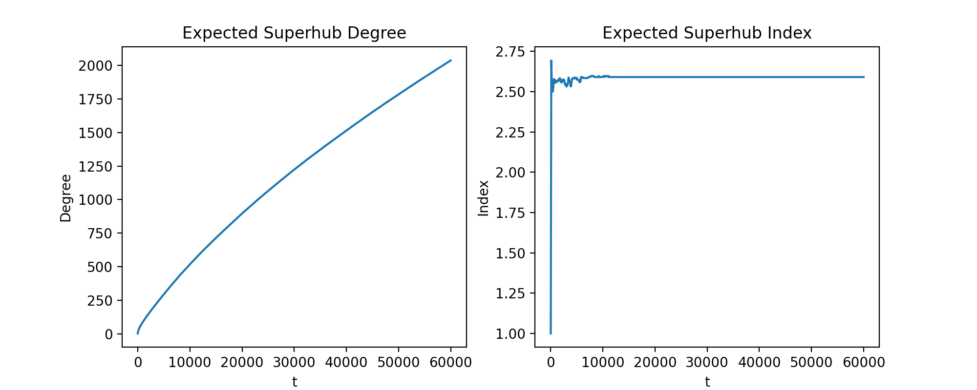 Superhub degree and index for \(m=2\). The log–log plot shows \(\deg(v_{\mathrm{SH}}) \approx \sqrt{2}\, t^{2/3}\).
Problem 4 (degree gap and second-order growth). Let \(v_{(2)}(t)\) be the vertex with second-largest degree (ties broken arbitrarily). Prove a nontrivial separation
\[\deg_t(v_{\mathrm{SH}}) - \deg_t(v_{(2)}(t)) \to \infty,\]and quantify the asymptotic size of the gap. For \(m=2\), justify the observed “two-scale” behavior where non-superhub degrees grow like \(t^{1/3}\).
Height and diameter
For \(m=1\), \(G_t^{(1)}\) is a tree, so height rooted at (say) vertex \(1\) is well-defined; for \(m>1\) the graph is cyclic, so we track diameter and distance to the superhub instead. Empirically, EPAN trees appear to have sublogarithmic height.
Problem 5 (sublogarithmic height/diameter). For \(m=1\), let \(H_t\) be the height of \(G_t^{(1)}\) rooted at vertex \(1\). Prove that \(H_t = o(\log t)\) with high probability, or determine its sharp order (e.g. \(\log t/\log\log t\), \((\log t)^\beta\), …). For \(m=2\), formulate and prove an analogous bound for \(\mathrm{diam}(G_t^{(2)})\).
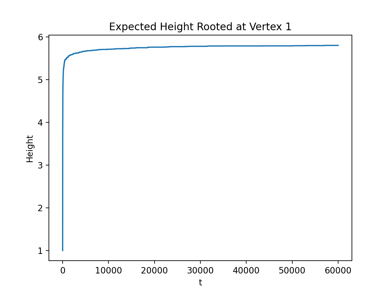 Height of the EPAN tree rooted at vertex \(1\), strictly sublogarithmic — contrast with the logarithmic height of BA preferential attachment.
Degree distribution and non-scale-free behavior
A striking qualitative difference from BA preferential attachment: EPANs are not scale-free. The degree sequence shows visible gaps, and for \(m=2\) the empirical distribution often shows two distinct “peaks” instead of a single power law — a phenomenon first noted by Adami et al.
Problem 6 (characterize the degree distribution). Let \(D_t\) be the degree of a uniformly sampled vertex of \(G_t^{(m)}\). Determine whether \(D_t\) converges in distribution as \(t \to \infty\) and, if so, identify the limit law. Explain and prove the mechanism behind the observed degree gaps / two-peak structure.
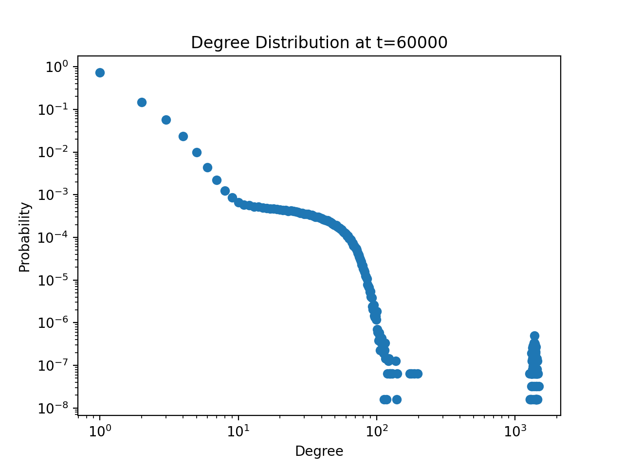
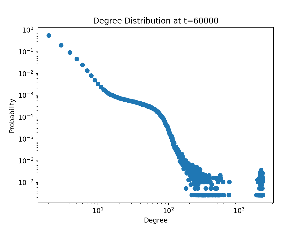 Empirical degree distributions for \(m=1\) (left) and \(m=2\) (right); note the two-peak structure at \(m=2\).
Eigenvector centrality dynamics
Because attachment probabilities are proportional to Perron–Frobenius eigenvector entries, understanding how those entries evolve is essential. Empirically, high-degree vertices can decrease in expected eigenvector centrality over time, while the superhub maintains substantially larger centrality than everyone else.
Problem 7 (monotonicity / drift of eigenvector entries). Let \(v_t \in \mathbb{R}^{t+m}\) be the \(\ell_1\)-normalized Perron–Frobenius eigenvector of \(A(G_t^{(m)})\). Fix an “old” index \(i\) and study \(\lbrace v_t(i)\rbrace _{t \ge i}\): is \(\mathbb{E}[v_t(i)]\) decreasing in \(t\) for large \(t\)? Can one prove concentration, or a deterministic asymptotic profile, for \((v_t(i))_{i \le t}\)?
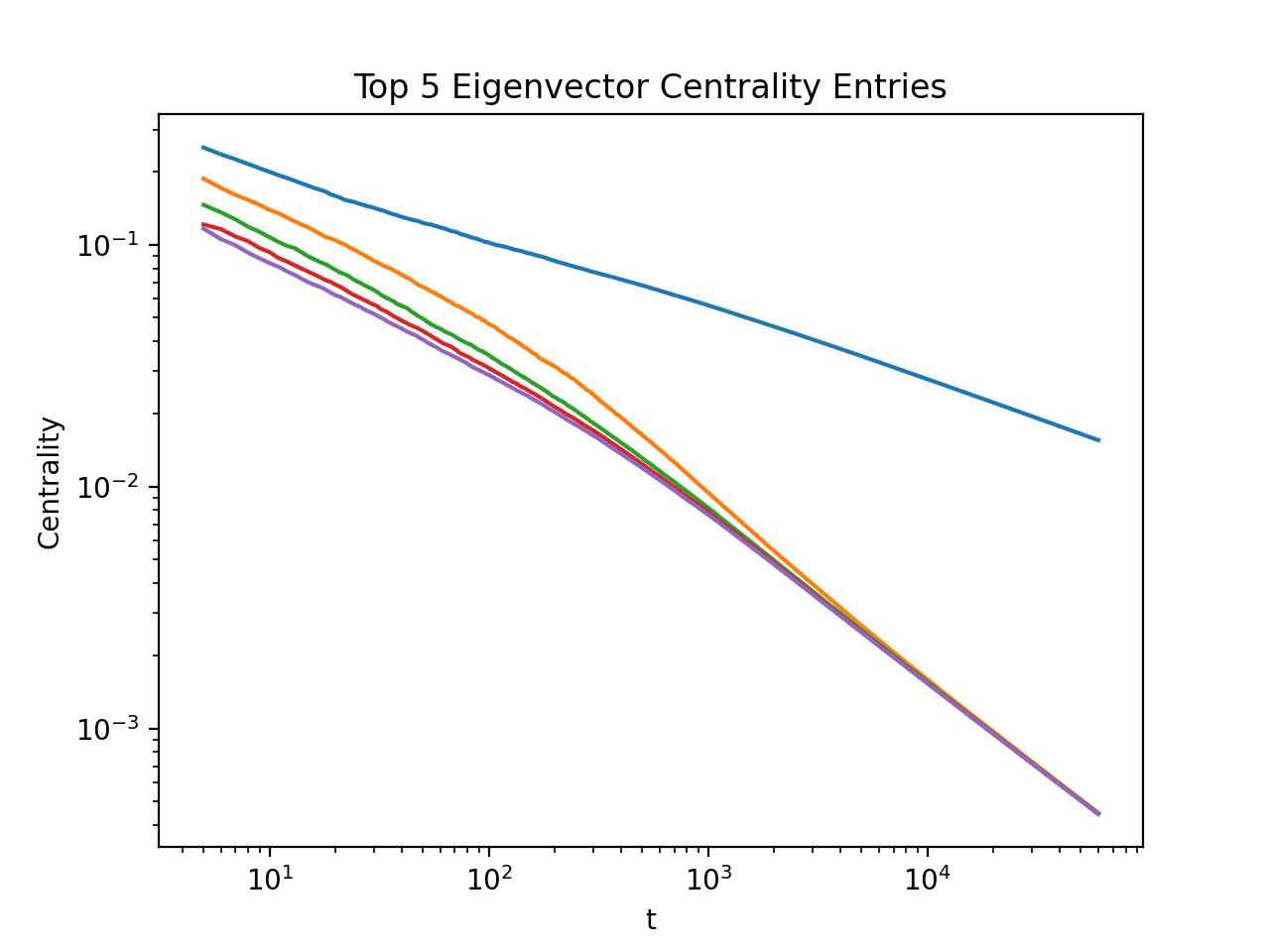
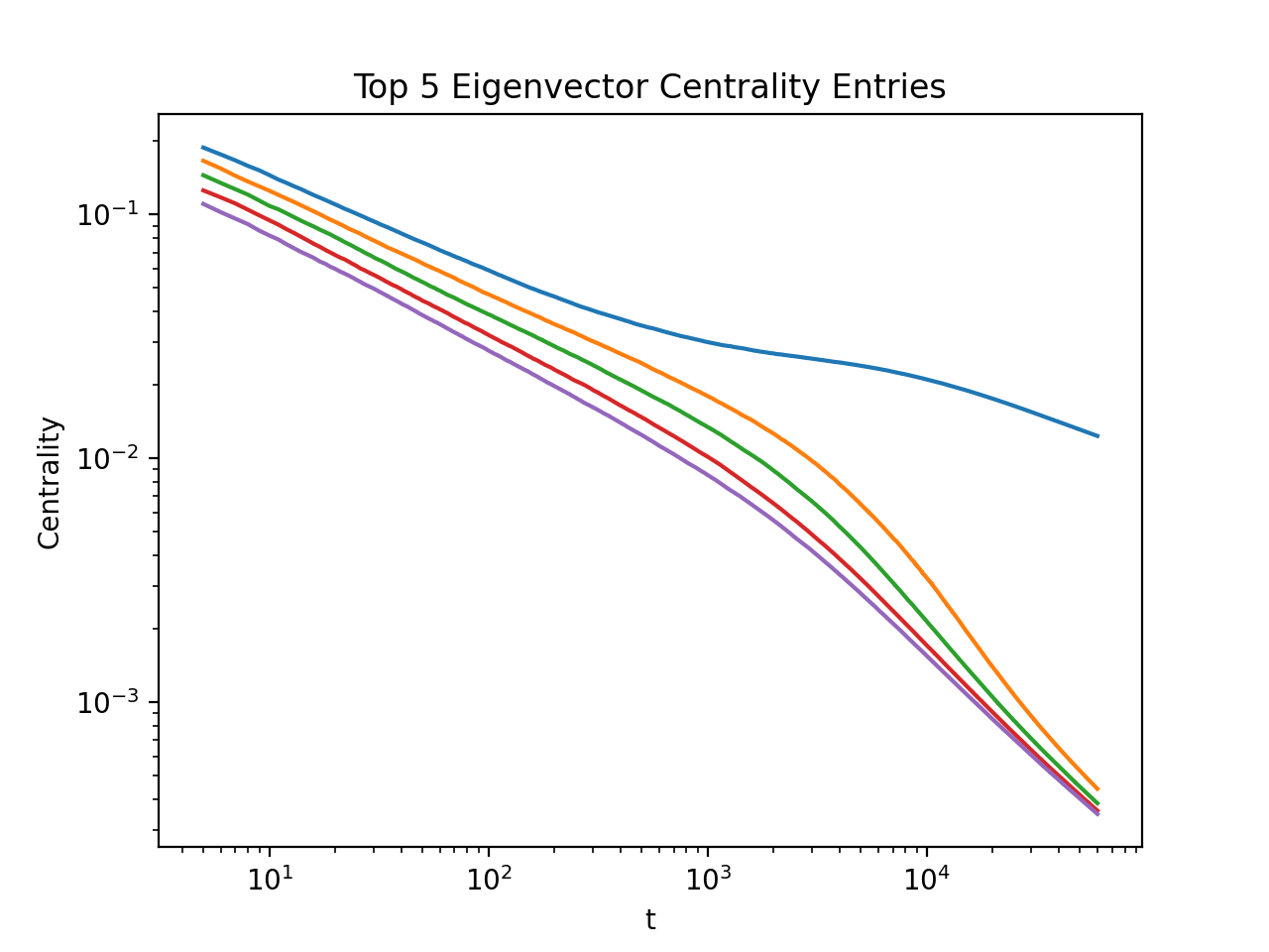 Greatest 5 eigenvector centralities for \(m=1\) (left) and \(m=2\) (right). The superhub (max-degree) index does agree with the maximal eigenvector index, which shows large separation from the rest.
Problem 8 (degree–centrality relationship). Quantify the relationship between \(\deg_t(v)\) and \(v_t(v)\): prove inequalities of the form \(c_1\, f(\deg_t(v)) \le v_t(v) \le c_2\, g(\deg_t(v))\), or identify regimes where degree is a poor proxy for eigenvector centrality in EPAN.
Theoretical results
Three structural features point toward possible proof strategies for the problems above.
Feature 1: complete spectrum dependency
At step \(t\), given the \(m\) vertices the new vertex attaches to (encoded as a bit vector \(a_t \in \lbrace 0,1\rbrace ^t\)), the new Perron–Frobenius eigenvector depends on the entire spectrum of \(A_t\) — not just the top eigenpair.
Proposition. Let \(A_t\) be the adjacency matrix of \(G_t\), with orthonormal eigenbasis \(\lbrace v_1,\dots,v_t\rbrace\), eigenvalues \(\lbrace \lambda_1,\dots,\lambda_t\rbrace\), \(D_t = \mathrm{diag}(\lambda_1,\dots,\lambda_t)\), and \(Q_t = [v_1\ \cdots\ v_t]\). Then
\(A_{t+1} = \hat Q_{t+1}^{T} \left[\begin{array}{cc} D_t & Q_t^T a_{t+1} \\ (Q_t^T a_{t+1})^T & 0 \end{array}\right] \hat Q_{t+1}, \qquad \hat Q_{t+1} = \left[\begin{array}{cc} Q_t & 0 \\ 0 & 1 \end{array}\right].\)
Proof. Writing \(A_{t+1}\) in block form with \(A_t\), the new edge vector \(a_t\), and a zero corner,
\[A_{t+1} = \left[\begin{array}{c|c} A_t & a_t \\ \hline a_t^T & 0 \end{array}\right],\]direct block-matrix multiplication with \(\hat Q_{t+1}\) gives the result. \(\blacksquare\)
So \(A_{t+1}\) is similar (via \(\hat Q_{t+1}\)) to the matrix
\[\left[\begin{array}{cc} D_t & q \\ q^T & 0\end{array}\right], \qquad q = Q_t^T a_t,\]in the basis \(\lbrace (v_1,0),\dots,(v_t,0),e_{t+1}\rbrace\) — visibly involving every eigenpair of \(A_t\). In fact the characteristic polynomial can be written out explicitly:
Proposition.
\(\chi_{A_{t+1}}(\lambda) = (-\lambda)\prod_{i=1}^t (\lambda_i - \lambda) + \sum_{i=1}^t -q_i^2 \prod_{j \ne i}^t (\lambda_j - \lambda), \qquad q = Q^T a_t.\)
Proof. Define the bordered determinants
\[K_0 = \begin{vmatrix} \lambda_1 - \lambda & & & q_1 \\ & \ddots & & \vdots \\ & & \lambda_t - \lambda & q_t \\ q_1 & \cdots & q_t & -\lambda \end{vmatrix}, \qquad K_i = \begin{vmatrix} \lambda_{i+1}-\lambda & & & q_{i+1} \\ & \ddots & & \vdots \\ & & \lambda_t - \lambda & q_t \\ q_{i+1} & \cdots & q_t & -\lambda \end{vmatrix},\]and \(R_i = (-1)^{t-i+3} q_i \cdot (\text{cofactor expansion along the first row}) = -q_i^2 \prod_{j=i+1}^t (\lambda_j - \lambda)\), so that \(K_0 = K_1 + R_1\) with \(K_t = -\lambda\). This gives the recurrence \(K_i = (\lambda_{i+1}-\lambda)K_{i+1} + R_{i+1}\), and unrolling it from \(K_t\) back to \(K_0\) yields
\[K_0 = (-\lambda)\prod_{i=1}^t(\lambda_i - \lambda) + \sum_{i=1}^t -q_i^2\prod_{j\ne i}^t (\lambda_j-\lambda). \qquad \blacksquare\]Feature 2: distance and spectral properties
Elementary arguments give weak inequalities showing that vertices closer together have closer eigenvector centralities.
Proposition (height–spectral radius inequality). Let \(A\) be an adjacency matrix satisfying Perron–Frobenius, with spectral radius \(\rho\). For any two vertices \(i,j\),
\[\left(\frac{1}{\rho}\right)^{d(i,j)} \le \frac{v_i}{v_j} \le \rho^{d(i,j)}.\]For EPANs, this gives an a.s. bound relating diameter \(d_n\), spectral radius \(\rho_n\), and the superhub / minimum eigenvector entries:
\[d_n \overset{\text{a.s.}}{\le} \frac{\left\lvert \log\!\big(v_{\mathrm{SH}}(n)/v_{\min}(n)\big) \right\rvert}{\log(\rho_n)}\](the same bound holds with height in place of diameter when \(m=1\)).
Proof. Induct on \(d(i,j)\), which is finite since \(G\) is connected. If \(d(i,j)=1\): from \(\rho v = Av\), \(\rho v_i = \sum_{i \rightsquigarrow j} v_j\) (adjacency is \(0/1\)). By Perron–Frobenius, \(v_j \ge 0\) for all \(j\), so \(\rho v_i \ge v_k\) whenever \(i \rightsquigarrow k\). By symmetry in \(i,k\), \(\frac1\rho \le \frac{v_i}{v_k} \le \rho\) for \(d(i,k)=1\). Chaining this inequality along a path of length \(d(i,j)=n\) gives \(\left(\frac1\rho\right)^{d(i,j)} \le \frac{v_i}{v_j} \le \rho^{d(i,j)}\). The EPAN bound follows by maximizing \(\frac{v_i}{v_j}\) and \(d(i,j)\), then taking logs and rearranging. \(\blacksquare\) <!–
Feature 3: blurred locality
Let \(G_t = (V,E)\), and suppose a new vertex \(u_{t+1}\) attaches only to \(u_k\), forming \(G' = (V \cup \lbrace u_{t+1}\rbrace ,\, E \cup \lbrace (u_k,u_{t+1})\rbrace )\). For every \(u_i\) with \(d(u_i, u_{t+1}) > 23\), the normalized centrality of \(u_i\) decreases:
\[\left(\frac{v_i}{\sum_{j=1}^t v_j}\right)_{G} \le \left(\frac{v_i}{\sum_{j=1}^{t+1} v_j}\right)_{G'}.\]For the special case of a path graph \(P_T\) (root \(u_0\)), appending one vertex changes \(u_0\)’s centrality by
\[\Delta = \sqrt{\frac{2}{T+1}} \sin\!\left(\frac{\pi}{T+1}\right)\Big/Z_G \;-\; \sqrt{\frac{2}{T+2}}\sin\!\left(\frac{\pi}{T+2}\right)\Big/Z_{G'},\]where \(Z_G = \sqrt{\tfrac{2}{T+1}}\sum_j \sin\!\left(\tfrac{j\pi}{T+1}\right)\) and \(Z_{G'} = \sqrt{\tfrac{2}{T+2}}\sum_j \sin\!\left(\tfrac{j\pi}{T+2}\right)\) — an explicit case where a purely local edge addition provably ripples outward through the whole eigenvector, motivating the name “blurred locality.” –>
Numerics of EPAN simulation
Given seed graph \(G_0 = K_{m+1}\), a simulation up to time \(T\) proceeds as:
- $$G \gets K_{m+1}$$
- for $$t \gets 1$$ to $$T$$:
- $$v \gets$$ getPFEigenvector($$G$$)
- $$u_1,\dots,u_m \gets$$ RandomSample(values $$=\{1,\dots,t+m\}$$, weights $$=v_1,\dots,v_t$$, number $$=m$$)
- $$V, E \gets G$$
- $$G \gets \big(V \cup \{t+m+1\},\ E \cup \{t+m+1\} \times \{u_1,\dots,u_m\}\big)$$
Most of the work is in computing the Perron–Frobenius eigenvector at every step. \(K_{m+1}\) has \(\binom{m+1}{2}\) edges, and each of the \(T\) steps adds \(m\) more — so although \(A_t \in \mathbb{R}^{(t+m)\times(t+m)}\), it has only \(mt+O(1)\) edges (twice as many nonzero entries). We focus on \(m=1\) and \(m=2\) without worrying about scaling to large \(m\).
The eigenvalue problem
\(A\) is real, symmetric (undirected graph), and sparse. Two standard methods for the sparse symmetric eigenproblem are power iteration and Lanczos iteration; we use power iteration.
For a diagonalizable \(A \in \mathbb{R}^{n\times n}\) with \(\lvert\lambda_1\rvert \ge \lvert\lambda_2\rvert \ge \cdots \ge \lvert\lambda_n\rvert\) and eigenvectors \(\mathbf v_i\), write an arbitrary \(\mathbf x_0 = \sum_i \alpha_i \mathbf v_i\) and \(\mathbf x_i = A^i \mathbf x_0\). Then
\[\left\lVert \frac{\mathbf x_i}{\lambda_1^i} - \alpha_1 \mathbf v_1 \right\rVert = \left\lVert \sum_{j=2}^n \left(\frac{\lambda_j}{\lambda_1}\right)^{i} \alpha_j \mathbf v_j \right\rVert \le \left(\frac{\lambda_2}{\lambda_1}\right)^{i} \left\lVert \mathbf x_0 - \alpha_1 \mathbf v_1\right\rVert,\]so \(\mathbf x_i / \lambda_1^i \to \alpha_1 \mathbf v_1\) at rate \(\lvert \lambda_2/\lambda_1 \rvert < 1\): repeated multiplication by \(A\) converges to the Perron–Frobenius eigenvector (even from a bad initial vector, floating-point error alone perturbs it off any non-dominant eigenspace).
The \(m=1\) case is bipartite, which breaks this: \(\lvert\lambda_1\rvert = \lvert\lambda_2\rvert\), so naive power iteration doesn’t converge.
Proposition. If a graph \(G\) is bipartite, then for every eigenvalue \(\lambda\) of \(A\), \(-\lambda\) is also an eigenvalue.
Proof. Permute \(A\) into block form (the two partitions):
\[A = \left[\begin{array}{cc} 0 & B \\ B^T & 0 \end{array}\right].\]If \(v = (\mathbf v_1, \mathbf v_2)^T\) is an eigenvector for \(\lambda\), then \(Av = (B\mathbf v_2, B^T \mathbf v_1)^T = \lambda(\mathbf v_1, \mathbf v_2)^T\), and one checks directly that \(A(-\mathbf v_1, \mathbf v_2)^T = -\lambda(-\mathbf v_1,\mathbf v_2)^T\). \(\blacksquare\)
For \(m \ge 2\), \(K_{m+1}\) is not bipartite, so this issue never arises. For \(m=1\), we instead solve on the shifted matrix \(A + \sigma I\): since \((A+\sigma I)\mathbf v = (\lambda+\sigma)\mathbf v\), any \(\sigma > 0\) separates the shifted top eigenvalue enough for power iteration to converge, and we recover the eigenvector of \(A\) directly. Empirically \(\sigma = \rho_{t-1}/2\) works well. Warm-starting from \(\mathbf x_0 = (\mathbf v_{\max}^{t-1}, 1/t)^T\) (the previous step’s eigenvector, padded) converges in roughly 40 iterations.
Sparse matrix representations: CSR, COO, and DynamicCSR
With only \(2tm + o(1)\) nonzero entries in \(A_t\), sparse storage is essential for both memory and matrix–vector speed. We use a combination of two formats:
Compressed Sparse Row (CSR) stores the matrix row by row as one flat value[] array (nonzero entries only), a index[] array of column indices, and a pointer[] array marking where each row starts/ends:
| value array | \([3,5,6,7,1,2,4,9,8]\) |
| column indices | \([0,1,3,1,0,3,1,2,3]\) |
| row pointers | \([0,3,4,6,9,9]\) |
(for the matrix with rows \([3,5,0,6,0],[0,7,0,0,0],[1,0,0,2,0],[0,4,9,8,0],[0,0,0,0,0]\) — row \(i\)’s values live at value[pointer[i] : pointer[i+1]].)
CSR uses \(O(N_{nz})\) floats and is worth it whenever \(N_{nz} < \frac{mn-m-1}{2}\) — true here for large \(t\), since \(A_t\) is \((t+m)\times(t+m)\) with \(N_{nz}=2tm\). Matrix–vector multiplication in CSR is \(O(N_{nz})\), with the row-by-row structure giving good (sequential) memory access — though random access into the input vector \(v\) is still the dominant cost, since sparse matvecs are inherently memory-bound.
CSR’s weakness is column/edge insertion: appending a new column costs \(O(N_{nz}'\log N_{nz}')\) (transpose, insert a row, transpose back) — far too slow to repeat at every timestep.
Coordinate format (COO) stores each nonzero as an (row, column, value) triple. Matrix–vector multiplication is still \(O(N_{nz})\), but with more overhead than CSR (random access on both sides of the product, not just the input vector). Its advantage is edge insertion in \(O(\Delta N_{nz})\) — essentially free.
DynamicCSR. We combine the two: the bulk of \(A_t\) — everything except a small, recently-grown tail — is stored in CSR, while the actively growing edges are buffered in COO. New edges land in the COO block in \(O(m)\) time; every \(\tau\) steps the COO block is merged back into CSR (\(A_t \gets (A_{\mathrm{CSR}, t_1+t_2},\, A_{\mathrm{COO},0})\), reset the buffer, repeat). This keeps matrix–vector multiplication at \(O(N_{nz})\) with CSR-comparable overhead — the COO tail adds only \(O(\tau)\) extra cost — while making per-step edge updates \(O(m)\) instead of paying CSR’s full reallocate-and-shift cost on every step.
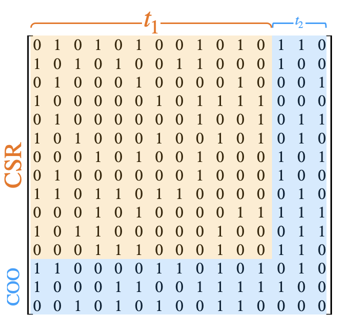 DynamicCSR: most of the matrix lives in CSR; the actively growing edge frontier is buffered in COO and periodically folded back in.
Conclusion
EPAN replaces BA preferential attachment’s local, degree-based rule with a global one driven by the Perron–Frobenius eigenvector, and that shift in mechanism shows up everywhere: a unique, persistent superhub with \(t^{2/3}\) degree growth and a visible gap to the rest of the network, sublogarithmic tree height instead of BA’s logarithmic height, a non-scale-free (gapped, sometimes two-peaked) degree distribution instead of a power law, and eigenvector-centrality entries that can decrease over time even as the underlying vertex’s degree grows. We formalized these observations as eight open problems, and made partial theoretical progress: a full-spectrum dependency result showing that (unlike degree-based models) the entire spectrum, not just the top eigenpair, feeds into every update; a height–spectral-radius inequality bounding diameter (or height, for \(m=1\)) via the spectral radius and the superhub-to-minimum centrality ratio; and an explicit “blurred locality” example showing a single local edge addition provably perturbs eigenvector centrality arbitrarily far away.
On the computational side, simulating EPAN at meaningful scale means solving a sparse symmetric eigenvalue problem at every step. We used power iteration with warm starts, handled the \(m=1\) bipartite obstruction via a matrix shift, and built the DynamicCSR hybrid format to keep matrix–vector products fast while making per-step edge insertion cheap.
The natural next step is to bring in existing results on low-rank perturbations of random matrix spectra and adapt the martingale techniques used for degree-based preferential attachment — which don’t transfer directly, since EPAN’s preference function can’t easily be written in terms of degree alone. EPAN’s dependence on global spectral information is exactly what makes it richer than degree-driven models, and exactly what will require new techniques to analyze rigorously.
-
Cover image is taken from Adami et. al. ↩