OscNet: Learning the Delayed Oscillator in a Finite Linear Subspace
May 20, 2026
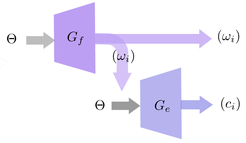
Abstract. We parametrize the solution map of the delayed oscillator, which takes the oscillator’s parameters to a solution. The approximate solution lives in a \(d\)-dimensional linear subspace spanned by \(\cos(\omega_i t)\) and \(\sin(\omega_i t)\), \(i = 1, \dots, d\), and two MLPs learn the best subspace and the coordinates in it, respectively.
The result is not satisfactory and is open for future projects.
Acknowledgement This project is kindly supported by Elfarouk Harb who provided numerous feedbacks and A100 credits on Delta NCSA.
The Delayed Oscillator
The delayed oscillator is a minimal model of the El Niño–Southern Oscillation (ENSO). It describes a single scalar \(h(t)\), such as the east-Pacific mean thermocline depth anomaly, by
\[\frac{dh}{dt} = a\,h(t) - b\,h(t - \delta) - r\,h(t)^3,\]with four parameters \(\Theta = (a, b, r, \delta)\):
- \(a > 0\), the strength of the local positive feedback;
- \(b > 0\), the strength of the delayed negative feedback, which acts after a lag \(\delta\);
- \(r > 0\), the nonlinear damping that keeps the oscillation bounded.
Although it looks like a single first-order ODE, the system is infinite-dimensional: the state at time \(t\) is the whole history of \(h\) on \((t - \delta, t)\). Its solutions are typically asymmetric, non-sinusoidal oscillations (see the experiments below).
The Learning Task
Let \(\mathcal{Y} = \mathcal{Y}((0, \infty); \mathbb{R})\) be a separable Banach space of functions of time, and let
\[G: \mathbb{R}^4 \to \mathcal{Y}, \qquad \Theta = (a, b, r, \delta) \mapsto h\]be the solution map, which sends the parameters to the solution (from a fixed initial history). Evaluating \(G\) requires a numerical DDE solve for every new \(\Theta\). The goal of this project is to learn \(G\): a network that takes \(\Theta\) and returns the whole solution at once.
Model
Architecture of the Oscillator Net
The oscillator net \(G_\theta: \mathbb{R}^4 \to \mathcal{Y}\) parametrizes \(G\),
\[G_\theta = \operatorname*{argmin}_{\theta} \int_{\Theta} \int_0^\infty \big(G(\Theta)(t) - G_\theta(\Theta)(t)\big)^2\, dt\, d\Theta,\]by projecting the solution onto a finite-dimensional subspace. It has two parts:
- the frequency net \(G_f(\Theta) = (\omega_1, \dots, \omega_d)^\top\), which chooses the subspace \(W = \operatorname{span}\lbrace\cos(\omega_i t), \sin(\omega_i t)\rbrace_{i=1}^d\);
- the energy net \(G_e(\Theta; \omega_1, \dots, \omega_d) = (\underbrace{c_1, \dots, c_d}_{\cos}, \underbrace{c_{d+1}, \dots, c_{2d}}_{\sin})^\top\), which gives the coordinates in \(W\).
The prediction is
\[\tilde y(t) = \sum_{i=1}^d c_i \cos(\omega_i t) + c_{i+d} \sin(\omega_i t).\]The subspace dimension \(d \in \mathbb{N}\) is a hyperparameter. \(G_f\) and \(G_e\) are MLPs with \(\tanh\) activations, width 48 and 3 hidden layers.
Physics-Informed Loss
Since \(\tilde y\) is a linear combination of sines and cosines, its derivative is available in closed form and the physics loss needs no automatic differentiation. For a training sample \(((a, b, r, \delta), y)\),
\[\mathcal{J}_{\text{physics}} = \frac{1}{t_{\max} - \lceil\delta\rceil} \sum_{\substack{t = \lceil\delta\rceil \\ \text{step } \Delta t}}^{t_{\max}} \Big( a\tilde y(t) - b\tilde y(t - \delta) - r\tilde y(t)^3 - \sum_{i=1}^d \omega_i\big(c_{i+d}\cos(\omega_i t) - c_i \sin(\omega_i t)\big) \Big)^2,\]where \(\Delta t\) and \(t_{\max}\) are set by the grid of the numerical solver.
Data Generation
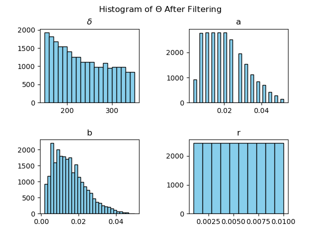
The data is generated with a custom Heun’s-method solver. We only simulate parameters \(\Theta = (a, b, r, \delta)\) for which the delayed oscillator actually oscillates:
Proposition (Vallis1) With \(\alpha := b/a < 1\), the delayed oscillator is oscillatory (unstable) only if
\(a\delta > \sqrt{\alpha^2 - (3\alpha - 2)^2} \cdot \arccos\left(\frac{3\alpha - 2}{\alpha}\right).\)
Experiments
Proposed Architecture
We test the model on 10 random samples.
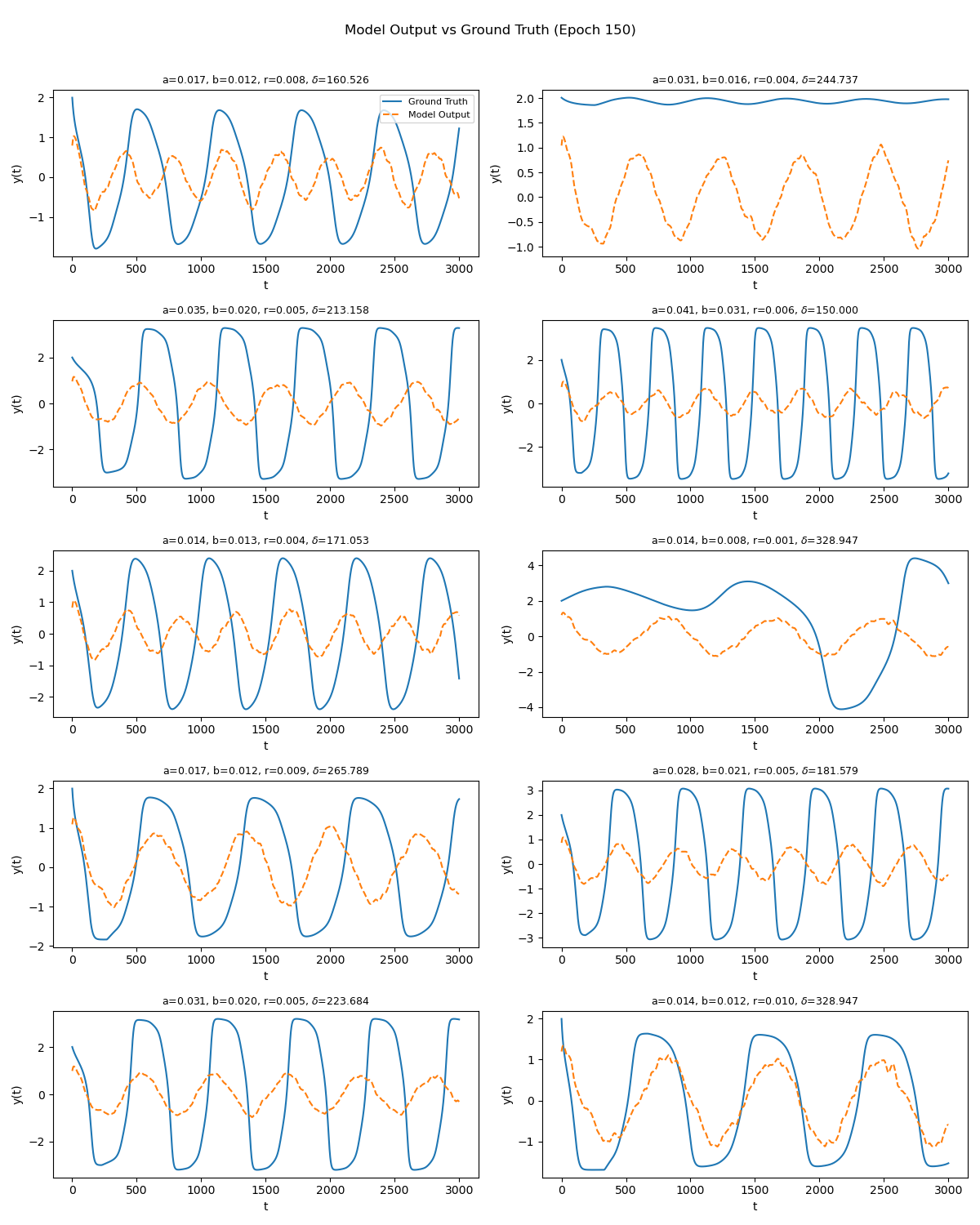
The model learns the general dependence of the frequency on \(\Theta\): the period is roughly that of the ground truth. It fails badly, however, at capturing the asymmetric shape of the oscillation, since its output is essentially sinusoidal. It also avoids large amplitudes, which suggests the output is more an average than a robust fit.
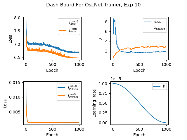
Throughout training, \(\mathcal{J}_{\text{physics}}\) dominates \(\mathcal{J}_{\text{data}}\), consistent with the output closely resembling a physically feasible oscillator.
Decoupled Architecture
We also tried a simpler architecture with no coupling between \(G_f\) and \(G_e\): \(G_e\) no longer takes the frequencies as input. The results are similar to those of the proposed architecture.
Conclusion
Two observations:
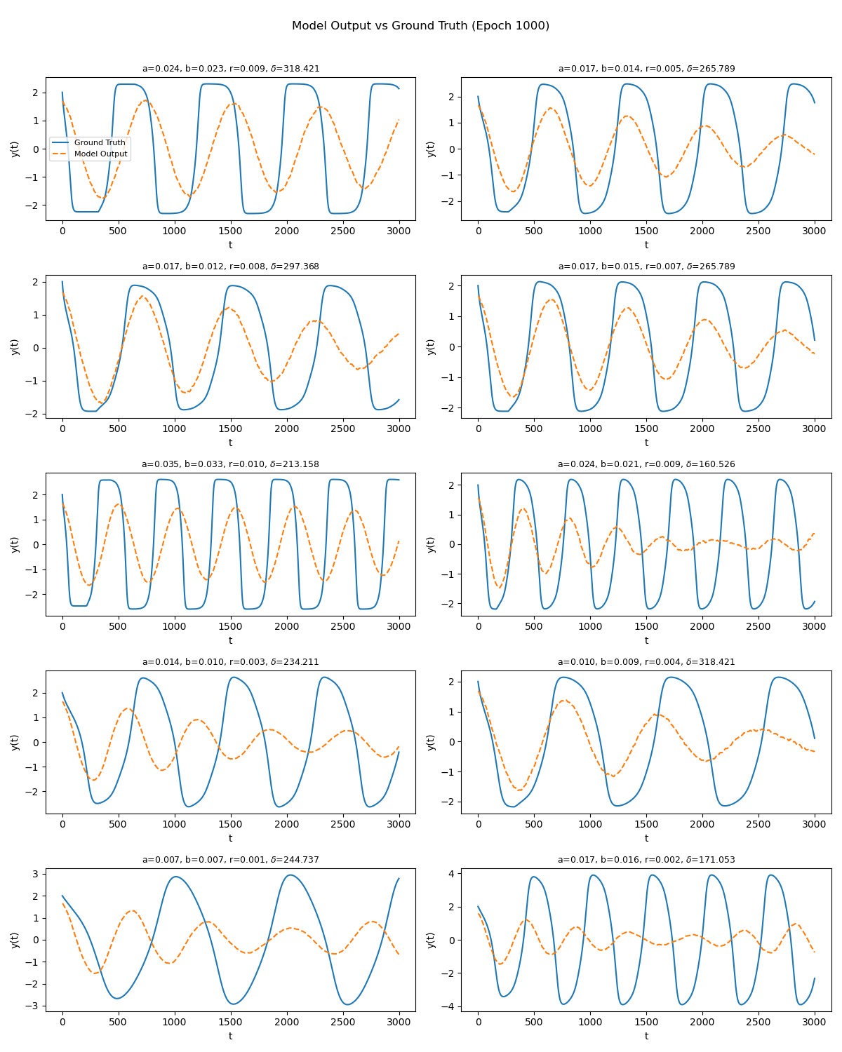
- The predictions are centered and do not capture high-amplitude oscillations.
- The decoupled model performs about as well as the coupled one.
Together they suggest that the current architecture does not model the delayed nonlinear system; it acts as a mean-finder that averages the training samples. Observation 2 also means the intended information flow, with \(G_f\) finding the subspace and \(G_e\) the coordinates, is not happening, since the decoupled model does as well, if not better.
Due to time constraints only about 30 experiments were run; a systematic grid search is needed to confirm that the architecture fails.
Another culprit may be sampling density. All data comes from a grid search, and with 4 parameters the grid is necessarily coarse, so each parameter has low variability in the data. Non-dimensionalization could help: with
\[\hat\delta = a\delta, \qquad \alpha = \frac{b}{a}, \qquad \hat h = h\sqrt{\frac{r}{a}},\]the delayed oscillator becomes
\[\frac{d\hat h}{d\hat t} = \hat h - \alpha\,\hat h(\hat t - \hat\delta) - \hat h^3,\]which has only two parameters. This costs physical interpretability, though: the substitution drops a degree of freedom, so \((a, b, r, \delta)\) cannot be recovered from \((\alpha, \hat\delta)\).
AI Disclaimer
Claude Code wrote the Julia scripts for simulating the shallow-water model. All other code and scripts, the LaTeX formatting and the TikZ figures are the author’s. Claude Code was also sometimes used to debug the training pipeline.
Gemini (3.5 Flash) proposed making the frequencies \(\lbrace\omega_i\rbrace\) an output of the model rather than a hard-coded hyperparameter. Initially, the subspace was fixed and only the coordinates were learned with an MLP.
-
G. K. Vallis, Atmospheric and Oceanic Fluid Dynamics, 2nd ed., Cambridge University Press, 2017. ↩