Learning Barotropically Unstable Zonal Jet with Spherical Neural Operator
June 1, 2026
Acknowledgements:
- This research project is supervised by Dr. Gan Zhang.
- Training and simulation is done with the
L40SGPUs on thekeelingcluster of the ATMS department at UIUC as well as theA100GPUs on theNCSA Deltacluster.
Overview
Spherical Fourier Neural Operators have been proven to be a powerful architecture to model real world climate dynamics. However little attention was given to benchmark the architecture with classical numerical testcases such as the Galewsky testcase, which consists of a barotropically unstable zonal jet flow in a shallow water system. Since neural operators learn the time-stepping map of a system between current and next state which is invariant to the input state, we propose the following workflow use idealistic testcase to verify the generalizability of neural operators. The SFNO model is trained on numerical data with ERA5 initial condition at 500hPa, and a initial condition similar to Galewsky testcase is used as a out-of-distribution input. The workflow can be generalized to other models and classical testcases, and it also serves as an ideal setup to pursue interpretability.
Background
Shallow Water Equation
We work with the vorticity form of SWE:
where \(\zeta\) is the relative vorticity, \(\delta\) is the divergence and \(\Phi\) is the geopotential.
Since we are on the periodic domain \(SO(2)\) psuedospectral methods are very natural to carry out. Specifically we use the following algorithm to generate training dataset:
- Input: $$(\hat\delta_t, \hat\zeta_t, \hat\Phi_t)$$
- Resolve Problem 1 (pull back to physical space): $$(\delta_t, \zeta_t, \Phi_t) \gets \mathrm{ivSHT}(\hat\delta_t, \hat\zeta_t, \hat\Phi_t)$$
- Resolve Problem 2 (closedness of the vorticity form): $$(u_t, v_t) \gets \mathrm{ivSHT}\left[-\frac{a}{l(l+1)}(\hat\delta_t, \hat\zeta_t)\right]$$
- Compute tendency:
- Absolute vorticity flux: $$\mathbf{F_v} = (\zeta+f)(u,v)$$
- Mass flux: $$\mathbf{F_m} = \Phi(u,v)$$
- Back to spectral space (in torch-harmonics,
vSHTreturns coefficients for (vort, div) in that order): $$V_v, D_v \gets -\frac{l(l+1)}{a}\,\mathrm{vSHT}(\mathbf{F_v})$$ $$V_m, D_m \gets -\frac{l(l+1)}{a}\,\mathrm{vSHT}(\mathbf{F_m})$$ - $$\partial_t \hat\zeta_t = D_v - \mathrm{sSHT}\!\left(\Phi + \frac{u^2+v^2}{2}\right)$$
- $$\partial_t \hat\delta_t = -V_v$$
- $$\partial_t \hat\Phi = -D_m$$
- Return: $$(\partial_t \hat\zeta,\ \partial_t \hat\delta,\ \partial_t \hat\Phi)$$
The Galewsky Testcase
The Galewsky testcase consists of a simple zonal flow:
\[u(\phi) = \begin{cases} 0 & \phi \leq \phi_0 \\ \frac{u_{max}}{C}\exp\left[ \frac{1}{(\phi-\phi_0)(\phi - \phi_1)}\right] & \phi_0 < \phi < \phi_1 \\ 0 & \phi \geq \phi_1 \end{cases}\]where \(C=\exp\left(-\frac{4}{(x_0-x_1)^2}\right)\) is a constant that normalize the value of \(u\) to \(u_{max}\) at the mid point.
The geopotential is then computed by solving the balance equation with the average height \(\overline h\) perturbed by a gaussian bump in advance.
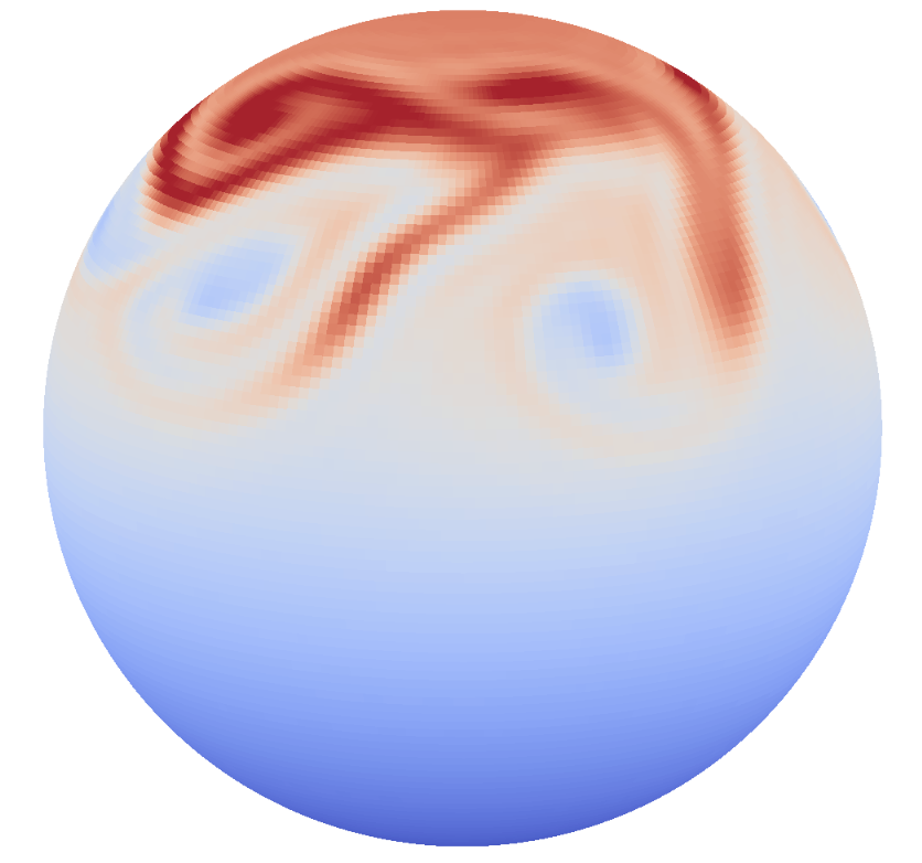
The ground truth evolution of the described initial condition contains a shift of flow regime from fast geostrophic adjustment to nearly balanced, slow flow that develops fine vortex structures.
Spherical Fourier Neural Operator
Neural opeartors solves a hyperbolic system like the SWE by parameterizing the solution map
Neural opeartors parametrizes time-stepping map
The time-stepping map can be defined as:
\[\begin{align*} G: \mathcal U(D;\mathbb{R}^d) &\to \mathcal U(D;\mathbb{R}^d) \\ u_{t} &\mapsto u_{t+\Delta t} \end{align*}\]where \(\mathcal U\) is a separable Banach Sapce containing functions from the domain \(D\) to climate variables \(\mathbb{R}^d\) with \(d\) being the number of channels.
The neural operator \(G_{\theta}\) minimizes the expectation of the \(L^p\) norm of the difference:
\[\theta = \mathrm{argmin}_{\theta}\mathbb{E}_{u \in \mathcal D} \left[ \| G_{\theta}(u) - G(u) \|_{L^p} \right]\]In ourcase, we take \(p=2\). The Spherical Fourier Neural Operator is a specfic instantiation of the neural operator \(G_{\theta}\) with \(\theta\) being convolution kernels in the fourier space.
Specifically, SFNO is consisted of sequential SFNO blocks:
SFNO is Theoretically just Global Convolution with Non-linear Activation on Sphere
A single SFNO block is the following composition:
\[u^{(j+1)} = \sigma(\mathcal F^{-1}(R\mathcal F(u^{(j)} + Wu^{(j)})))\]where \(u^{j}\) denotes the input for the \(j^{th}\) block. \(R\) is learnable convolution kernel. By the convolution theorem, pointwise multiplication is just global convolution.
The full SFNO model also consists of a lift and projection operator at the start and end of the sequence to raise the dimension of embedding states \(u^{(j)}\). In the following discussion we assume the embedding dimension to be \(d'=128\).
Learning SWE Dynamics using ERA5 dataset
Rather than creating synthetic flow patterns, we use real world ERA5 dataset data at 500hPa to generate initial conditions for the psuedospectral solver. Complete ERA5 global atmospheric reanalysis supports spectral data in Spherical Harmonics natively. Three variables relative vorticity, divergence and geopotential is directly obtained. To avoid aliasing, a exponential filter is used to truncate from T130 to T64. Using the truncated ERA5 data as initial states, the psuedospectral solver then generate 350 trajectories for 10 days.
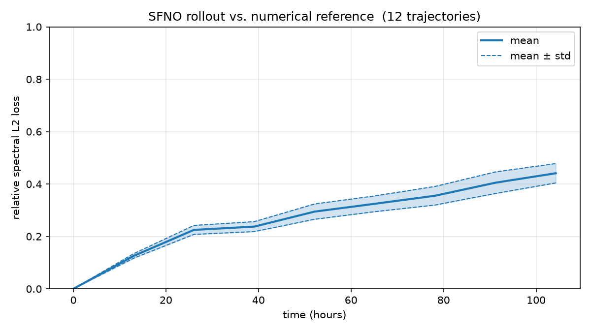
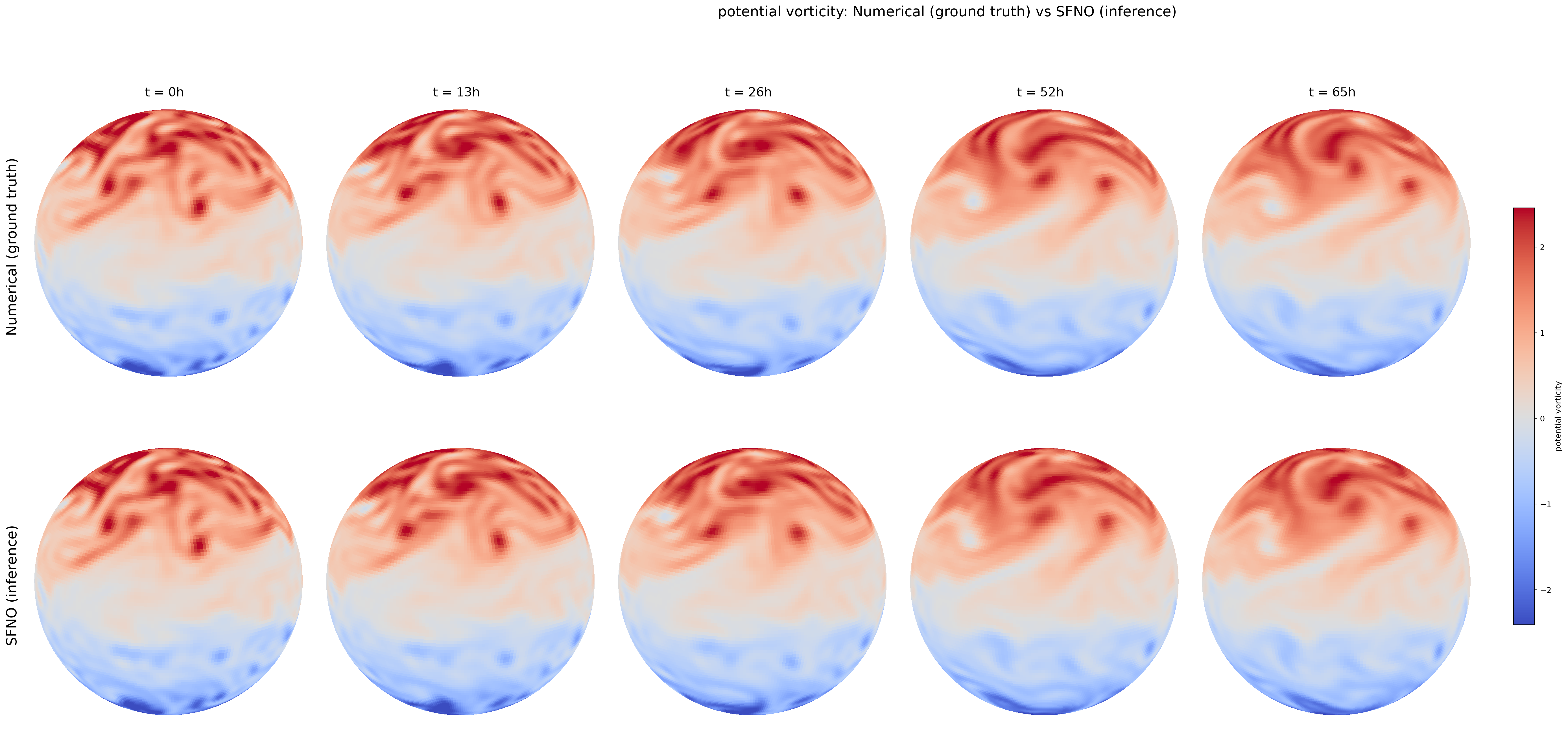
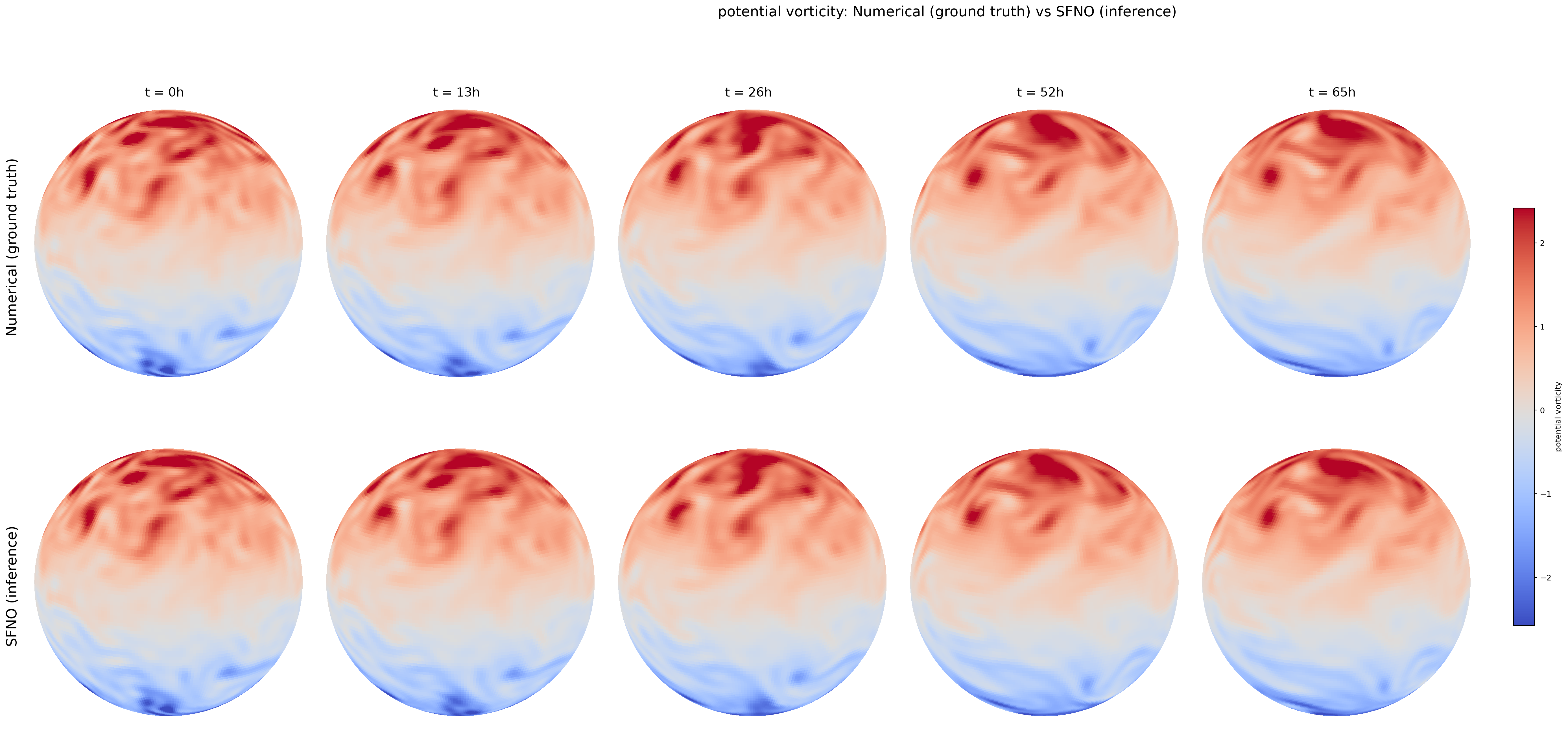
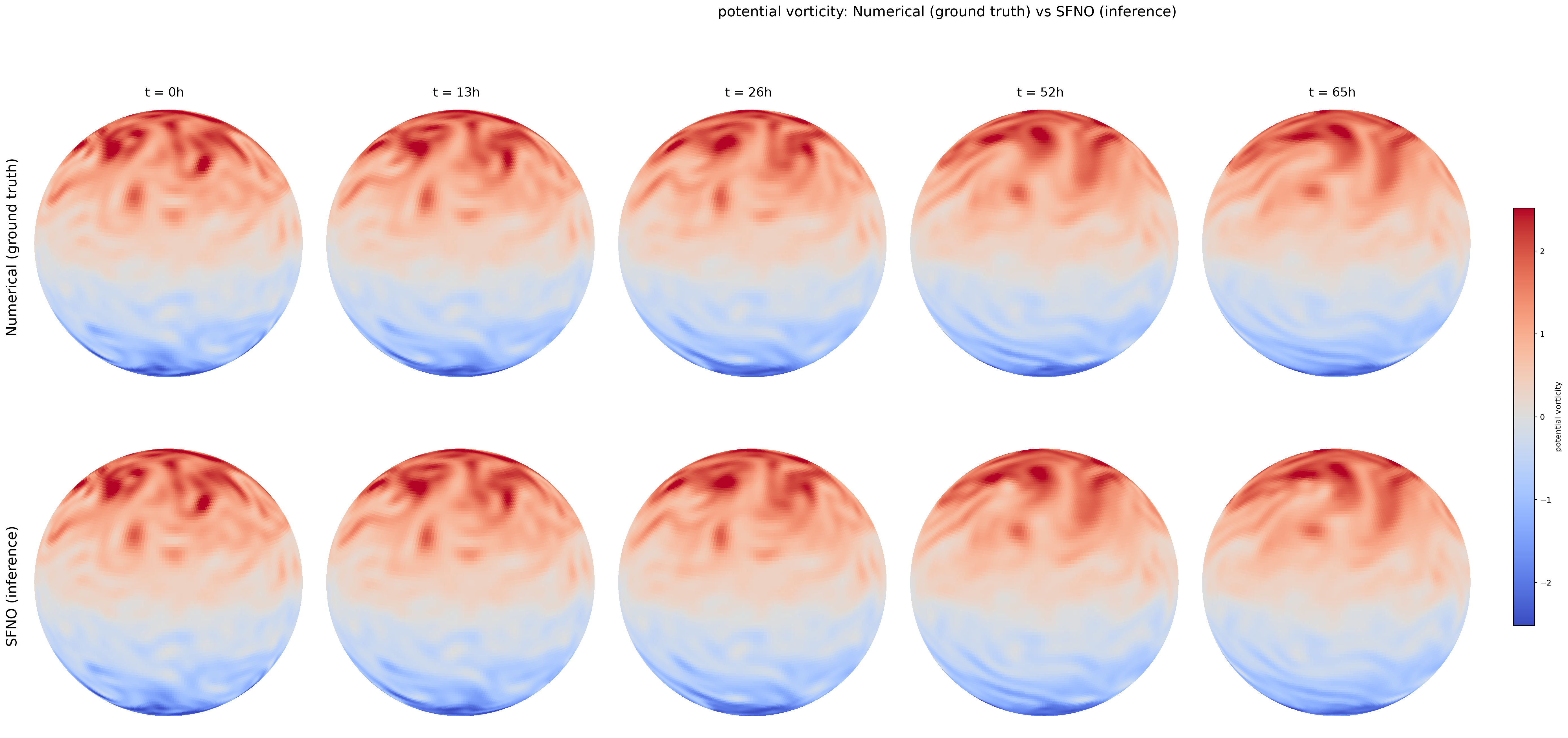
We train an SFNO model to predict the state of the dynamical system \(13\) hours ahead1 . The model has 4 SFNO blocks and an embedding dimension of 128. After training for 120 epochs , we obtain the following inference results on unseen ERA5 data:
Same example inferences are shown below.1
Generalizing to Galewsky Testcase
We use the trained model directly to inference Galewsky testcases with flow regime adjusted to the training dataset. Preliminary results show thet generalization fails:
-
We computed the largest possible timestep of the psuedospectral solver through CFL condition(primarily constrained by the gravity wave speed). This creates an contraint on the leadtime we can take. \(13\) hour is a reasonable value that is integral under the constraint. Small leadtime might lead to collpasing as the model attempt to learn the identity mapping. ↩ ↩2